SHAP values are a model-agnostic method to quantify the contribution of any given feature to a model’s prediction. They offer both local (per prediction) and global (overall) interpretations.

Shapley values

SHAP values have their roots in game theory, specifically in Shapley values. Imagine a group of players collaborating to achieve a payout. The Shapley value is a method to find out how to fairly distribute the total earnings among the players. Or the blame, if the payout was negative!

A core concept of Shapley values is coalitions: given \(n\) players, a coalition is a subset of the players. Another concept is the characteristic function, \(v: 2^N \rightarrow \mathbb{R}\), which returns the total payout for any given coalition (its worth). Here, \(N\) is the set of all players. The last concept is the Shapley value itself, the amount \(\phi_i\) that player \(i\) receives. It is computed as the average of the marginal contributions of player \(i\) to all possible coalitions that do not include it. More formally, for a game \((v, N)\):

\[\phi_i(v) = \sum_{S \subseteq N \setminus \{i\}} \frac{|S|!\; (n-|S|-1)!}{n!} (v(S\cup\{i\})-v(S))\]

These values satisfy four key properties, which collectively ensure fair attribution: efficiency, symmetry, dummy player, and additivity.

Efficiency

The grand coalition is the coalition of all players, \(N\). Efficiency means that the sum of all Shapley values equals the value of the grand coalition, i.e., the entire payout is distributed among the players:

\[\sum_{i \in N} \phi_i(v) = v(N)\]

Symmetry

Two players \(i\) and \(j\) are symmetric if their marginal contribution to any coalition not containing either player is the same. That is, if \(v(S \cup \{i\}) = v(S \cup \{j\})\) for any coalition \(S \subseteq N \setminus \{i, j\}\), then symmetry implies that players \(i\) and \(j\) receive the same Shapley value: \(\phi_i(v) = \phi_j(v)\).

Dummy player

If a player \(i\) does not change the value of any coalition they join (i.e., \(v(S \cup \{i\}) = v(S)\) for all \(S \subseteq N \setminus \{i\}\)), they are a dummy player. The dummy player property states that such a player’s Shapley value is 0.

Additivity

If two games with characteristic functions \(v_1\) and \(v_2\) are combined into a new game \(v_1 + v_2\) (where \((v_1+v_2)(S) = v_1(S) + v_2(S)\) for any coalition \(S\)), the Shapley values are additive:

\[\phi_i(v_1+v_2) = \phi_i(v_1) + \phi_i(v_2)\]

SHAP values

Machine learning models like linear regression are interpretable, as the model parameters indicate how each input feature contributes to the prediction. However, many complex models like neural networks or random forests are less directly interpretable: their output is a complex, non-linear combination of the input features. SHAP values (Lundberg and Lee, 2017) provide a framework to quantify the contribution of each feature to a specific prediction for any model. SHAP stands for SHapley Additive exPlanations, highlighting their connection to Shapley values.

Intuitively, SHAP values quantify how much each feature’s presence changes the prediction. Some features will have a negative contribution (pushing the prediction lower) and others a positive contribution (pushing the prediction higher). The sum of a feature’s SHAP value and a baseline value (typically the average prediction) approximates the model’s output.

To establish the connection to Shapley values, we map the game theory concepts to the machine learning context:

The \(n\) players become \(n\) predictive features.
The game is the trained model.
The payout for a coalition of features is the model’s prediction when only those features are known.

The Shapley value \(\phi_i\) for feature \(i\) in this context is then calculated as:

\[\phi_i = \sum_{S \subseteq F \setminus \{i\}} \frac{|S|!\; (n-|S|-1)!}{n!} (f(\mathbf{x}_{S\cup\{i\}})-f(\mathbf{x}_S))\]

where \(\mathbf{x}_S\) is the input datapoint including only the features in \(S\); \(F\) is the set of all features; \(n\) is the total number of features; and \(f_S\) is the model trained only on the features in set \(S\). However, this naïve approach is very computationally intensive, since it’d require retraining \(2^n\) models, one per possible coalition. (See a worked out example here.) SHAP values get around re-training models by approximating the effect of feature subsets using conditional expectations: \(f(\mathbf{x}_S) = \mathbb{E}[f(X) \mid X_S = \mathbf{x}_S]\). In other words, we fix the features that are in \(S\) to the sample values, and average over the predictions when sampling the remaining features from the dataset.

Simplified features: We use \(\mathbf{x}\) for the features in the original space \(\chi\), a vector of length \(n\). The SHAP theoretical framework uses a simplified feature vector \(\mathbf{x}' \in \{0,1\}^m\), where \(m\) is the number of simplified features (which can be different from \(n\)). \(x'_j = 1\) indicates that simplified feature \(j\) is “present” in a coalition, and \(x'_j = 0\) indicates it is “absent”. The simplified features are more useful for interpretation. For instance, if \(\mathbf{x}\) represented the individual pixels of an image, \(\mathbf{x}'\) could represent the presence of the “super pixels” that form a cat, grass or the sky. A mapping function \(h_\mathbf{x}: \{0,1\}^m \rightarrow \chi\) links the simplified representation back to the original feature space. For \(\mathbf{x}' = \mathbf{1}\) (all simplified features present), \(h_\mathbf{x}(\mathbf{1}) = \mathbf{x}\). For other \(\mathbf{x}'\), \(h_\mathbf{x}(\mathbf{x}')\) represents the original instance with features corresponding to \(x'_j=0\) appropriately handled (e.g., replaced by baseline values). Note that \(h_\mathbf{x}\) is specific to the instance \(\mathbf{x}\) being explained.

That covers the Shapley part of SHAP; let’s now focus on the Additive exPlanation bit. The goal of SHAP is to obtain a local, additive explanation model \(g\) for each prediction \(f(\mathbf{x})\) using the simplified features \(\mathbf{x}'\):

\[g(\mathbf{x}') = \phi_0 + \sum_{j = 1}^m \phi_j \mathbf{x}'_j\]

where \(\phi_0\) is the expectation over all training examples \(\mathbb{E}[f(X)]\). \(g(\mathbf{x}')\) is a very easy to interpret function that we’ll use to explain \(f(\mathbf{x})\).

Since SHAP values are Shapley values, they meet all the properties specified above. But they also satisfy three additional properties that are desirable for model explainers.

Local accuracy

When all simplified features are present (\(\mathbf{x}' = \mathbf{1}\)), the explanation model \(g\) must equal the prediction \(f(\mathbf{x})\):

\[f(\mathbf{x}) = g(\mathbf{1}) = \phi_0 + \sum_{j = 1}^m \phi_j\]

Missingness

If a feature is missing, it deserves 0 attribution:

\[\mathbf{x}'_j = 0 \implies \phi_j = 0.\]

This is a required property to ensure that local accuracy has a unique solution.

Consistency

The consistency ensures that if a model \(f\) changes into another model \(f'\), such that a feature’s contribution doesn’t decrease, the SHAP values do not decrease either. Formally, if

\[f'(S) - f'(S \setminus \{i\}) \geq f(S) - f(S \setminus \{i\})\]

for all \(S \in F\), then \(\phi_i(f', \mathbf{x}) \geq \phi_i(f, \mathbf{x})\).

A visual example

Let’s understand SHAP values better by looking at an example. I trained a model that uses 10 clinical features (body mass index, cholesterol, age, and a few others) to predict a continuous measure of disease progression one year after baseline. For the purposes of this example, the model is treated as a black box whose input are the 10 features, and the output a real number.

Age	Sex	BMI	Blood pressure	…	Target
0.0380759	0.0506801	0.0616962	0.0218724	…	151
-0.00188202	-0.0446416	-0.0514741	-0.0263275	…	75
0.0852989	0.0506801	0.0444512	-0.00567042	…	141
…	…	…	…	…	…

SHAP values can be computed on the dataset used to train the model (train set) or on a holdout set. Using a larger dataset like the train set might provide a more stable picture of overall feature contributions learned by the model. However, if the train and test data come from different distributions, computing SHAP on the respective sets will likely yield different results.

The shap package

SHAP values are implemented in Python via the shap package. While I won’t be showing any code here, you can see the code that generated the figures here.

SHAP values provide local explanations, showing the contribution of each feature to a particular prediction. I computed the SHAP values describing the importance of each of the 10 variables for each of the 442 patients. These values represent the estimated impact of each feature on a prediction, relative to the average prediction. We can start by looking at the SHAP values for one patient, using a waterfall plot:

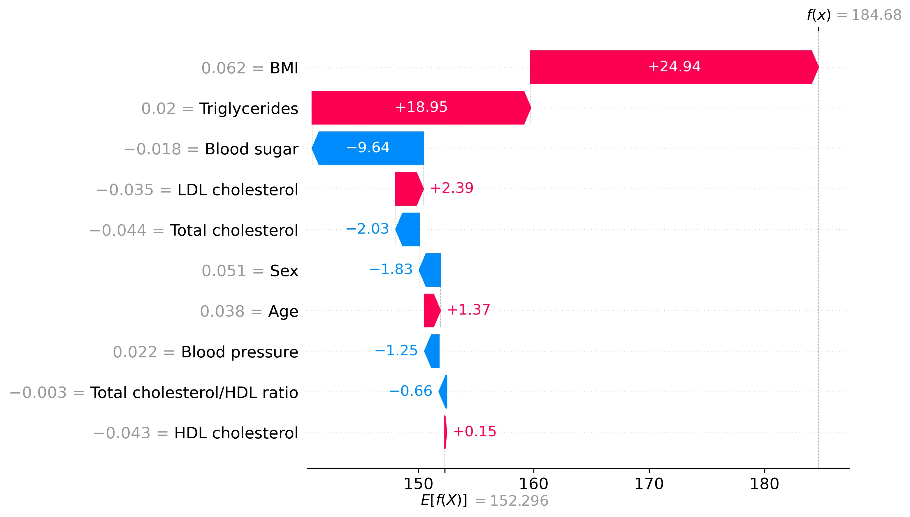
The waterfall plot shows how the prediction for this patient (186.53) departs from the average prediction over the training set (152.132). The difference (34.398) is the total change attributed by the model. As per the local accuracy property, the SHAP values for this instance sum up to this difference. The features are sorted by the absolute magnitude of their SHAP value. Features colored in pink push the prediction toward higher values, and features in blue toward lower values. We can see that, for this patient, the body mass index was the most important feature, contributing positively by 22.25.

We can visualize SHAP values for all 442 patients using a swarmplot:

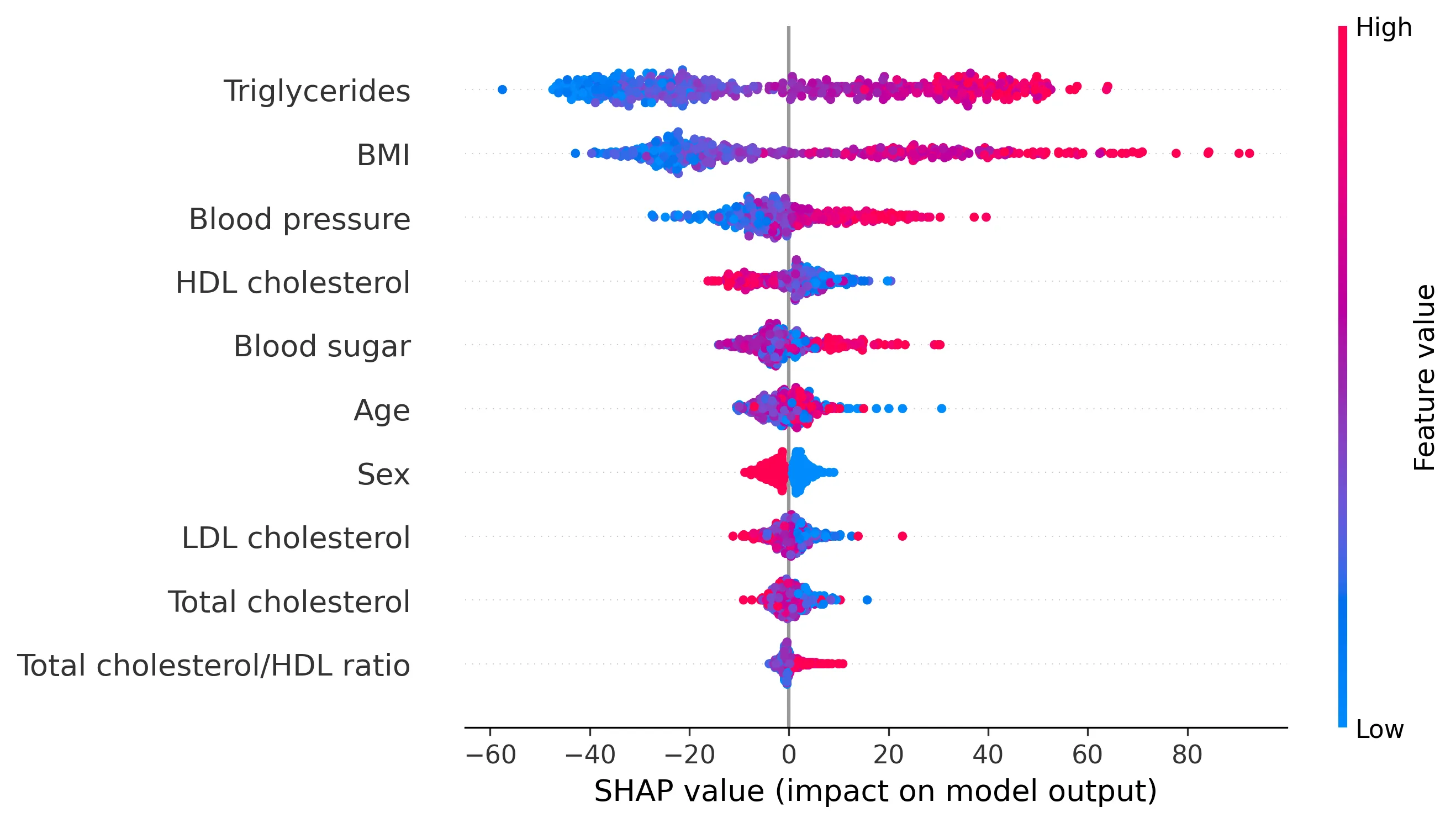
In the swarmplot, each point represents the SHAP value for a patient for a specific feature. Features are shown on the y-axis, and their corresponding SHAP values on the x-axis. As in the waterfall plot, features are sorted by their overall importance; and the color of each point indicates the feature value for that patient (pink for high, blue for low).

Global explanations can be derived by aggregating the local SHAP values over a dataset. A common global measure is the average absolute SHAP value for each feature:

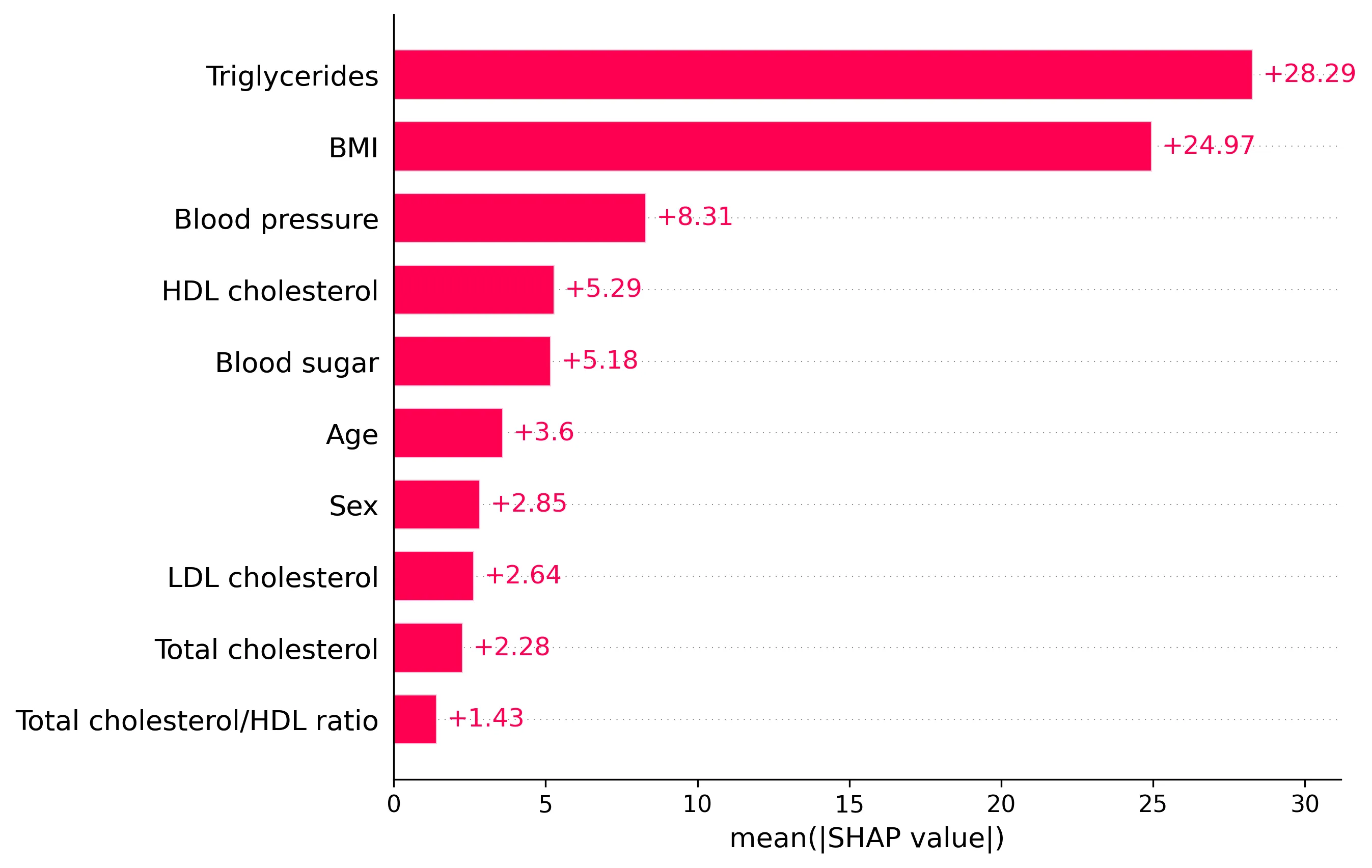
Plotting these averages shows which features have the largest impact on the model’s predictions on average across the dataset, providing a global measure of feature importance.

Lastly, SHAP values can be used for clustering. While traditional clustering groups data points based on their original feature values, clustering in SHAP space groups points based on how features contribute to the model’s prediction. This can be seen as a form of supervised clustering, as it leverages the model’s output (and indirectly the outcome it was trained on). Clustering SHAP values can reveal groups of instances where different sets of features drive the prediction.

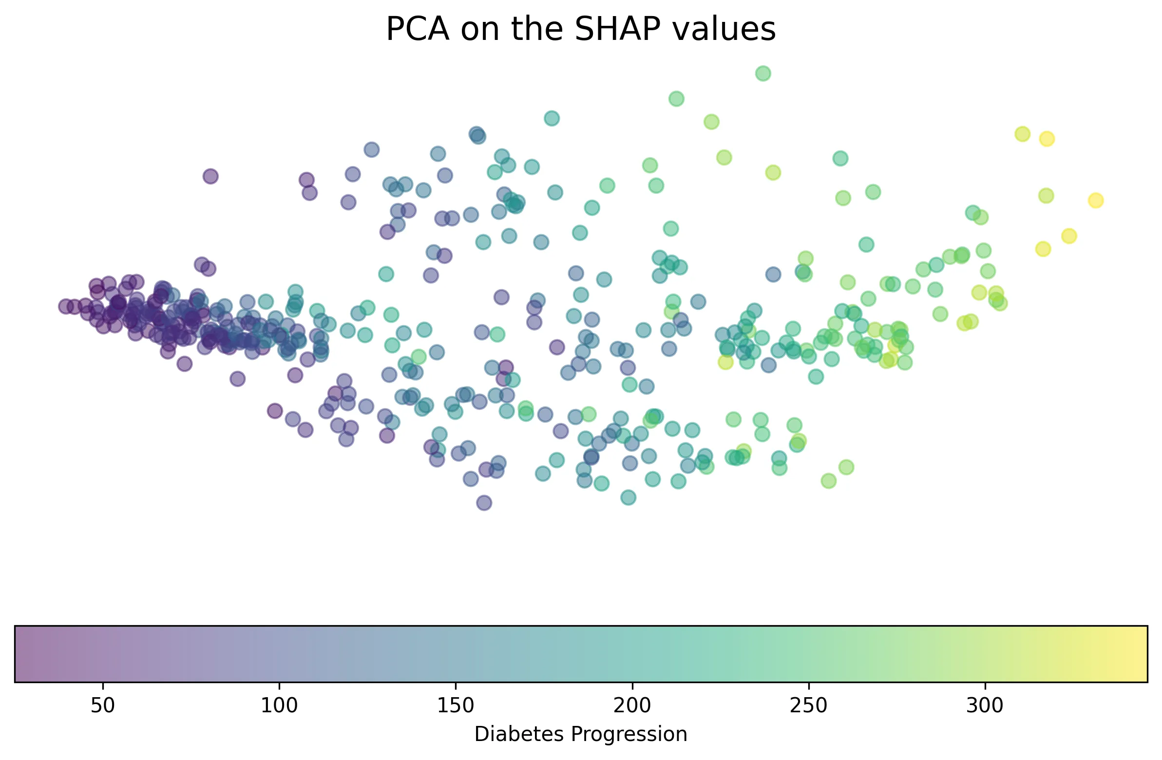
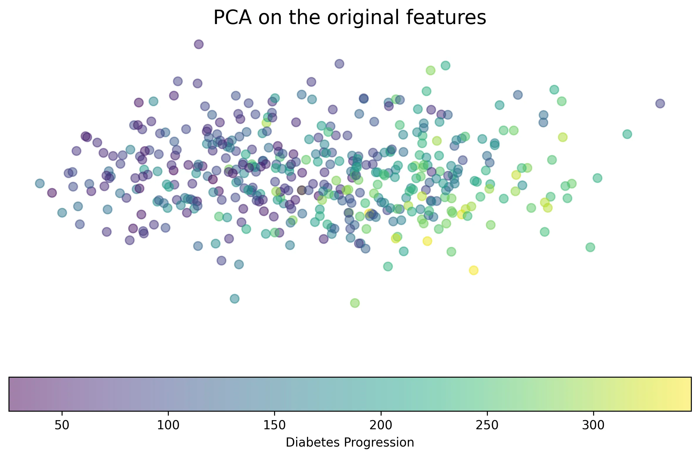
Applying PCA to the SHAP values (“supervised PCA”) and the original features (“unsupervised PCA”) for this dataset, we can visualize how instances are grouped.

Limitations

One key limitation of interpreting SHAP values is their behavior with highly correlated features. When features are strongly correlated, the model might arbitrarily use one over the others, or distribute importance among them. Consequently, the SHAP values for individual correlated features can become unstable or misleading, making it hard to disentangle their individual contributions.

Another point of consideration is feature interactions. While the fundamental Shapley value calculation inherently accounts for interactions (by averaging marginal contributions over different coalitions), the basic additive SHAP explanation model \(g(\mathbf{x}') = \phi_0 + \sum \phi_j \mathbf{x}'_j\) does not explicitly separate main effects from interaction effects. The \(\phi_j\) values represent the average contribution of feature \(j\), including its interactive effects, making their interpretation as pure “main effects” challenging when interactions are significant. However, SHAP can be extended to compute pairwise SHAP interaction values (\(\phi_{ij}\)) which explicitly quantify the interaction between features \(i\) and \(j\).

Finally, it’s important to remember that SHAP values explain how the model makes a prediction, not whether the prediction itself is correct. If the model is biased, overfit, or simply wrong for a given instance, the SHAP values will faithfully explain the mechanism behind that incorrect prediction. Measures like permutation feature importance, which rely on model performance metrics after feature perturbation, inherently account for the model’s correctness in their explanation.

Flavors of SHAP: the permutation approximation

Above I described the general approach to compute SHAP values. Unfortunately, it is very computationally intensive: exploring all possible coalitions is equivalent to exploring all \(2^m\) subsets of features. For that reason, different flavors of SHAP values have been proposed to make computations more efficient. I describe below the permutation approximation, a model-agnostic method to compute SHAP values \(\phi_i\). However, there are others specialized in specific model types, like Tree SHAP for tree-based models (e.g., random forests, gradient boosting) and Deep SHAP for deep learning models.

The permutation approximation approximates SHAP values by estimating the expected marginal contribution of each feature over many random permutations of the features. Let’s study the permutation approximation through a worked out example. We aim to explain a prediction \(f(\mathbf{x}_0)\). We have at our disposal a background dataset \(X_\text{bg}\), e.g., the whole training set, which we will use for sampling. For the sake of the example, our model only considers four (simplified) features: \(\mathbf{x}_0 = [x_{\text{age}}, x_\text{sex}, x_\text{BMI}, x_\text{BP}]\).

For each feature \(i\) that we want to explain:

Initializing a list to store the marginal contribution of each feature. In this example, I will focus on the contribution of the first feature, \(x_\text{age}\), so I will call this list just \(\text{list}_\text{age}\).
For \(K\) iterations:
1. A random ordering of the features is produced, e.g., \((\text{BP}, \text{age}, \text{BMI}, \text{sex})\), and a random sample \(\mathbf{z}\) is sampled from the background dataset \(X_\text{bg}\).
2. Create two synthetic examples: - \(\mathbf{x}_1 = (x_\text{BP}, x_\text{age}, z_\text{BMI}, z_\text{sex})\) - \(\mathbf{x}_2 = (x_\text{BP}, z_\text{age}, z_\text{BMI}, z_\text{sex})\) Note that the only difference between the two examples is the value of the age feature.
3. Compute the marginal contribution of the age feature as \(\delta = f(\mathbf{x}_1) - f(\mathbf{x}_2)\).
4. Append the marginal contribution to \(\text{list}_\text{age}\).
Approximate the SHAP value as the average marginal contribution: \(\phi_\text{age} \cong \frac{1}{K} \sum_i \delta_{i}.\)