How do vector databases work?
Finding similar documents in large collections
A big part of data science revolves around structured data, data that can be neatly organized into tables. We love tables: they can be easily sliced, diced, summarized, and filtered using SQL or another similar language. To check if an item exists in our table, we can do that quickly by querying for rows matching certain criteria.
However, large swaths of data can’t naturally fit in a table. This is the case with corpora of text, DNA sequences, or songs. In such cases, finding equal elements is still easy by, for instance, checking bit-wise equality. If we are feeling fancy, we might even do that efficiently using hash functions. However, approximate matching is even more important here. We want all the versions of our favorite song; all the pieces of news reporting on the same event; all the pictures containing a cat. This is where vector databases come in.
Formalizing the problem
Our goal is to find all documents in a collection of \(N\) items (like documents, images, or songs) that are similar, though not necessarily equal, to our query item. We will represent each item in a \(D\)-dimensional space. This problem can be decomposed into three subproblems:
- Embedding the items, that is, finding a \(D\)-dimensional, meaningful vector representation of each item
- Computing the similarity between items
- Efficiently finding the nearest neighbors of the query item
Let’s zoom in on each of these subproblems, then see how they come together in the context of large language models (LLMs) and retrieval-augmented generation (RAG).
The embeddings
Embeddings are vectors that meaningfully represent a piece of content—a song, a text, or a sequence of DNA. You can think of embeddings as the document’s coordinates in some arbitrary, very high-dimensional space. Related documents inhabit nearby regions of this space. If this sounds confusing, Simon Willison has a great introduction to embeddings that I recommend reading.

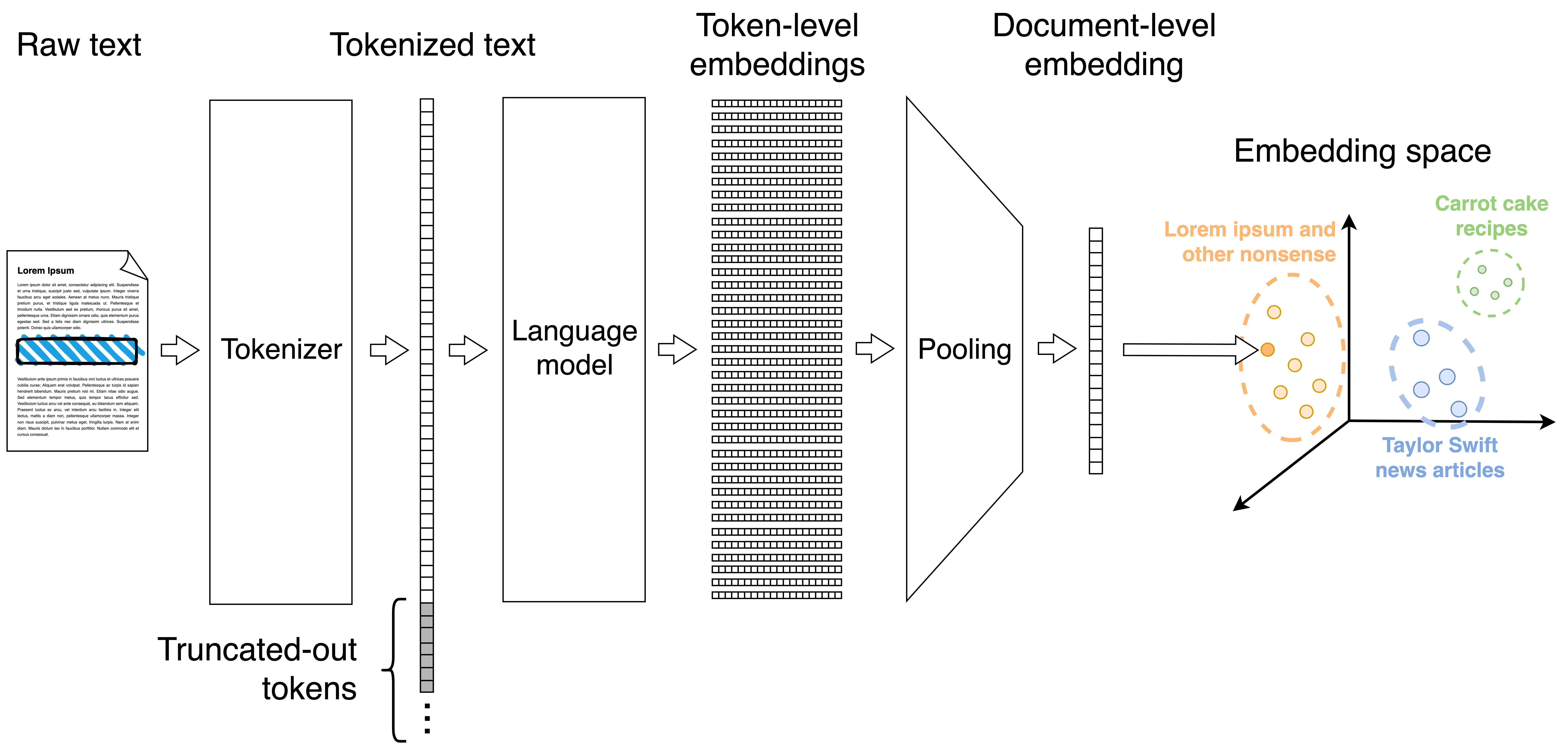
Embeddings are computed by a pre-trained model; they are often one of the intermediate representations of the model. This ensures two things. First, that the embeddings are meaningful. After all, the model learned a good representation of the data during training.
Embedding the items provides many advantages: where we once had amorphous blobs of unstructured data, we now have numerical representations that can be mathematically operated on. For instance, we can go from the 29 individual posts in my blog to a \(29 \times 384\) matrix of their embeddings. We can try to visualize their representation in two dimensions using UMAP, a popular dimensionality reduction technique:
We can see that posts with similar tags are neatly close to each other. But the embeddings offer a bit more nuance than that. Posts about statistical methods live near those about machine learning. The post about data structures lives between the posts related to Python and those discussing graphs.
Python implementation
from fastembed
from fastembed import TextEmbedding

# Small, high-quality model that is lightweight on CPU
MODEL_NAME = "sentence-transformers/all-MiniLM-L6-v2"

model = TextEmbedding(MODEL_NAME)

def compute_embeddings(
    texts: List[str], model: fastembed.text.TextEmbedding
) -> np.ndarray:
    """Compute embeddings using fastembed models."""

    embeddings = list(model.embed(texts))
    embeddings = np.array(embeddings)

    return embeddings
However, I just glossed over a very important detail: embedding a whole document is a bad idea. We can think of an embedding as lossy compression; and, since the dimensionality is fixed, cramming more content means losing more information. Not too unlike stuffing a novel into a tweet. That’s why many popular embedders are trained on sentences and short paragraphs, not on long texts. In fact, all-MiniLM-L6-v2 only used the first 256 tokens of each post and discarded the rest.
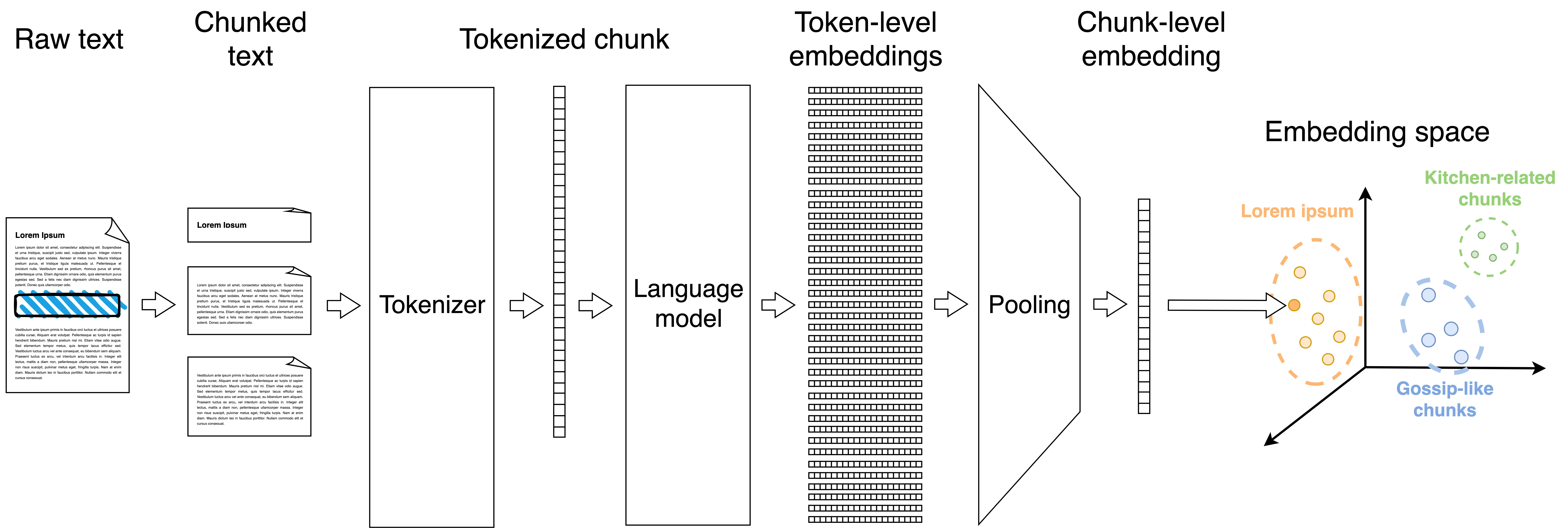
Instead of dealing with the whole document, it’s better to split each post into semantically coherent chunks (e.g., paragraphs) and then embed the chunks individually. Recursive character splitting is a simple strategy to get reasonably-sized chunks. It starts by splitting the document into paragraphs. Most paragraphs will be shorter than the model’s context window, and are ready to be embedded. But those that remain too long are further split into sentences; and, if these are still too long, it keeps going, splitting them into subsentences, words and, finally, into individual characters if absolutely needed. Additionally, it is a good idea to pad each chunk with content from the preceding and the following chunk to ensure that some context is also considered by the model.

Python implementation
def split_text(
    text: str,
    split_chars: List = ["\n\n", "\n", [". ", "! ", "? "], "; ", ", ", " "],
    max_size: int = 500,
) -> List[str]:
    """Recursively split text into chunks no larger than max_size."""

    if len(text) <= max_size:
        return [text]
    elif not split_chars:
        return [text[:max_size]]

    splitter = split_chars[0]
    splitter = (
        splitter if isinstance(splitter, str) else "|".join(map(re.escape, splitter))
    )
    splits = []

    for chunk in re.split(splitter, text.strip()):
        splits.extend(split_text(chunk, split_chars[1:], max_size=max_size))

    return splits
I applied this strategy to my 29 blog posts, obtaining 1,388 chunks of text. I then embedded each chunk individually. Here is the UMAP plot of the resulting embeddings:
The results here are now more nuanced. In general, the points are grouped by their post of origin, denoted by their color, which is a good sanity check. On the top right we find chunks coming from my posts on Python, which are understandably quite similar.
The distance measure
Now that we have a numerical representation of our items, we can start comparing them. But how do we define similarity?
If our goal was to find identical documents, an efficient solution would be relatively straightforward: hash them and see which ones fall in the same bucket. But that’s not the task we’ve embarked on. If the number of documents is large enough, eye-balling the UMAP plot is not an option either. We need a distance measure, a function whose inputs are two items and whose output is a real value telling us how far they are. The distance will be small when the two items are alike, and large when they are not. Analogously, we can define a similarity measure, which is inversely related to distance.
Many distance and similarity measures have been defined for different kinds of data. In the vector spaces in which our embeddings live, the most popular ones are:
| Measure | Formula | Meaning | Range |
|---|---|---|---|
| Cosine similarity | \(\frac {u \cdot v} {|u| |v|}\) | Extent to which $u$ and $v$ point in the same direction | \([-1, 1]\) |
| Dot product | \(u \cdot v\) | Same as cosine, but multiplied by the magnitude of $u$ and $v$ | \((-\infty, \infty)\) |
| Euclidean distance | \(\sqrt{\sum_i (u_i - v_i)^2}\) | Distance between the tips of $u$ and $v$ in Euclidean space | \([0, \infty)\) |
The cosine similarity is a common choice to measure semantic similarity of embeddings. The intuition is that vector direction matters more than magnitude—two documents about the same topic should be similar regardless of their length. Furthermore, in practice negative cosine similarities between embeddings are rare, so the range of interest is really \([0, 1]\).
Python implementation
def cosine_similarity(X: np.ndarray) -> np.ndarray:
    """Compute the cosine similarity matrix between the rows in X."""
    norms = np.linalg.norm(X, axis=1, keepdims=True)
    X_norm = X / (norms + 1e-8)  # Add epsilon to avoid division by zero
    return np.dot(X_norm, X_norm.T)
For instance, here is the similarity matrix between all 1,388 text chunks:
Nearest neighbor search
Let’s say we are interested in the 5 chunks most related to interpretable machine learning. A way to finding them is to compare the embedding of our query (Interpretable machine learning) against that of all my chunks. Here are the five chunks with the highest cosine similarity:
| Post title | Cosine similarity | Text sample |
|---|---|---|
| SHAP values | 0.514 | Machine learning models like linear regression… |
| SHAP values | 0.505 | - Interpretable Machine Learning: Shapley valu… |
| SHAP values | 0.403 | To establish the connection to Shapley values,… |
| SHAP values | 0.391 | Let’s understand SHAP values better by looking… |
| SHAP values | 0.388 | Global explanations can be derived by aggregat… |
I would say the search worked reasonably well!
However, this brute-force approach has a time complexity of \(O(D \cdot N)\), where \(D\) is the dimension of the embeddings (384) and \(N\) is the number of chunks (1,388). For large collections, this becomes prohibitively slow. That’s why we need approximate methods that can find good matches efficiently.
In the past, I described a method to find similar items using local-sensitivity hashing (LSH). The idea is to hash the items in such a way that similar items are likely to fall in the same bucket. This way, we can quickly scan over a corpus and find the items that are similar to our query. However, LSH has high memory requirements and requires careful parameter tuning. Here I will focus on hierarchical navigable small world graphs (HNSW) instead, a more modern method that is the backbone of vector databases. They build on two concepts: skip lists and navigable small world graphs.
Skip lists
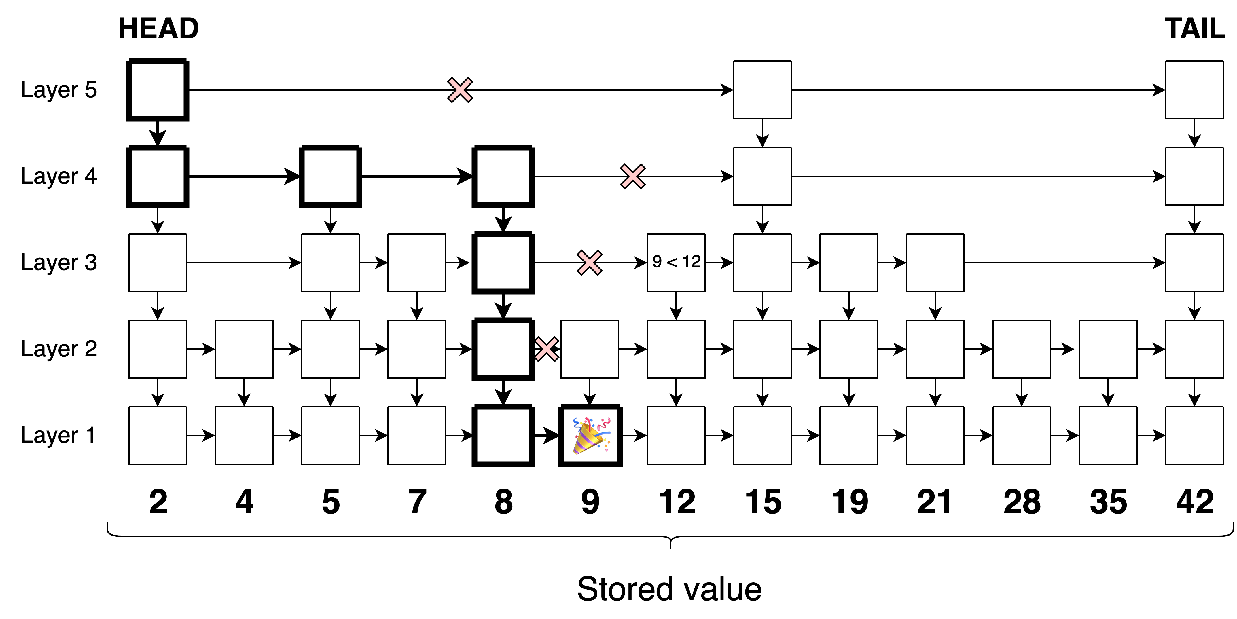
Skip lists are a data structure consisting of a set of linked lists, containing nested subsets of the items in the collection:

The topmost list contains only a few items, while the bottommost list contains all the items. Each item in a list points to the next item in the same list, and also to the next item in the lists below it. This allows us to quickly traverse the lists and find or insert items in logarithmic time with high probability.
Navigable small world graphs
Small world graphs are graphs with two key properties: small mean shortest-paths and high clustering coefficients. The classic example is the “six degrees of separation” phenomenon in social networks, where any two people are connected through at most six intermediate connections.
Navigable small world graphs extend this concept by ensuring we can find a path between any two nodes via a greedy strategy that chooses the neighbor closest according to a distance function. The key insight is that not all small world graphs are navigable: you need the right balance of local and long-range connections.
In a navigable small world graph:
- Local connections: each node connects to its immediate neighbors (high clustering); they are akin to local streets in a city.
- Long-range connections: some nodes have connections that “jump” across the graph (short paths); they are akin to highways connecting distant parts of the city.
- Greedy navigability: at each step, you can always find a neighbor that gets you closer to your target.
The challenge is constructing these graphs so that the greedy algorithm actually works. If you have too many random long-range connections, you might get stuck in local optima. If you have too few, the paths become too long. The magic happens when the probability of a long-range connection decreases with distance \(d\) in a specific way (roughly proportional to \(1/d^k\) where \(k\) is the dimensionality of the space).
The search algorithm
HNSW graphs combine the layered structure of skip lists with the navigability properties of small world graphs to create an efficient approximate nearest neighbor search algorithm.
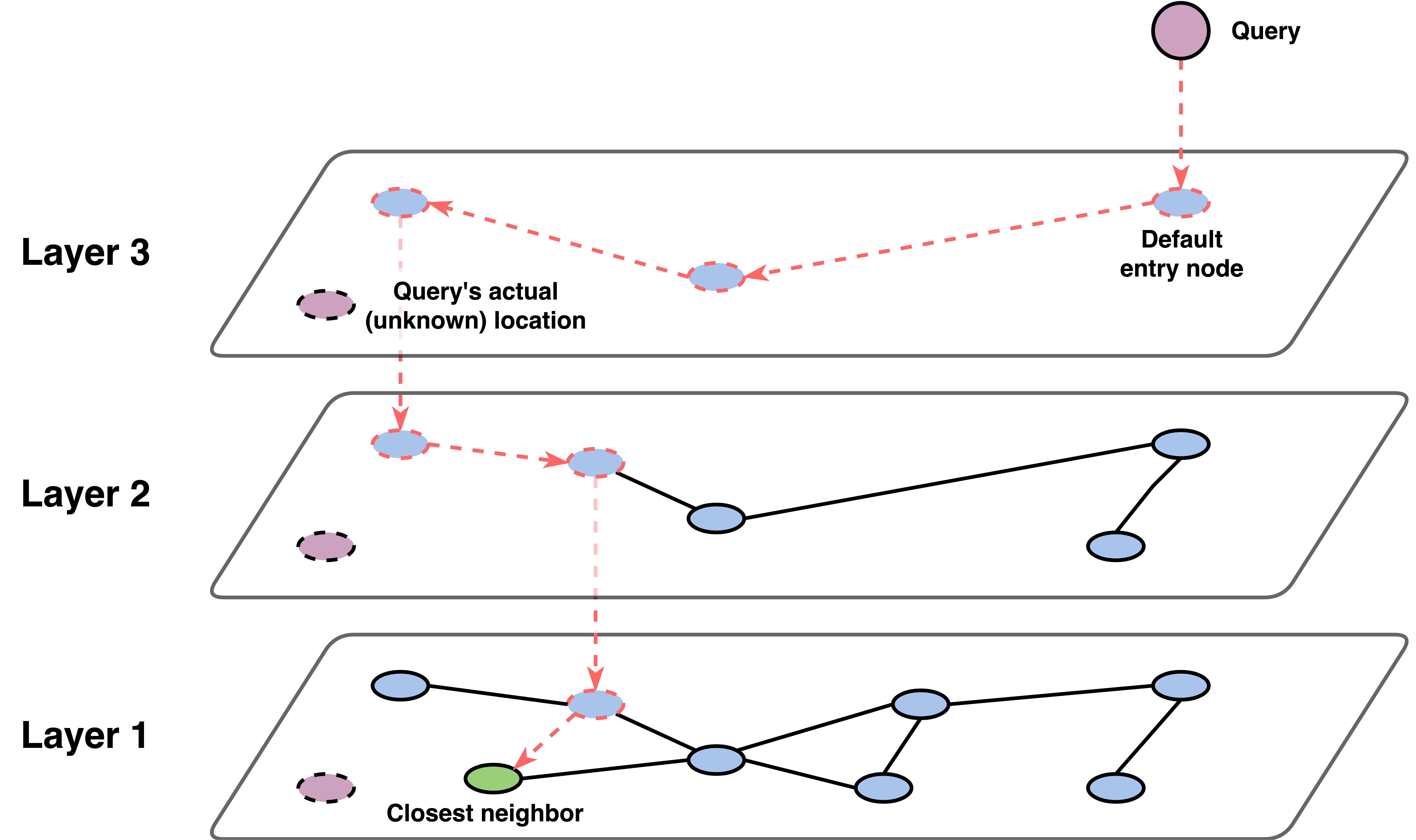
Like skip lists, HNSW graphs are organized in layers (typically 3-6 layers). The bottommost layer contains all the items in the collection, while the upper layers contain progressively fewer items. Each item has a randomly assigned maximum layer level, with the probability of being in a given layer following an exponential decay. This ensures that most items are in the lower layers, while only a few “hub” items exist in the upper layers,
Like navigable small world graphs, each item in a layer is connected to several of its nearest neighbors in the same layer. Additionally, items connect to themselves in lower layers, creating vertical connections that allow movement between layers.

The search process is what makes HNSW particularly effective:
- Start high: begin at the top layer with a default entry point
- Greedy descent: at each layer, greedily move to the neighbor closest to your query
- Layer transition: when you can’t improve further, drop to the next layer down
- Refine at bottom: perform a more thorough search in the bottommost layer
This multi-scale approach allows HNSW to quickly “zoom in” on the right region of the space. The upper layers provide coarse navigation (like highways), while the bottom layer provides fine-grained search (like local streets).
Vector databases
Vector databases like Qdrant are specialized in storing embeddings and finding the nearest neighbors of a query embedding. They do the latter via HNSW graphs, which they use as indexing structures. They are built incrementally: every time we add a new item to our collection, we update the graph. Graph building requires specifying some hyperparameters that affect its performance:
- M: the maximum number of connections per node (typically 12-48)
- efConstruction: the size of candidate set during construction (affects build quality vs. speed)
- ef: the size of candidate set during search (affects accuracy vs. speed)
The navigability property inherited from small world graphs is what makes this greedy strategy work: you can start from any entry point and confidently “walk” toward your query, finding good approximate neighbors without exhaustive search.
On top of fast nearest neighbor search, vector databases provide additional functionality like ACID transactions, filtering by metadata, versioning, and replication. They are optimized for high-dimensional data and can handle millions of items efficiently.
Why does this matter? LLMs and RAGs
Typically, an LLM leverages two sources of information to produce an output: its memory and the provided query. The LLM’s memory consists of large swaths of patterns learned during training and stored in its weights. The query is the user request, which gives the LLM relevant context, potentially additional information, and puts all those weights to find the most plausible answer. Vector databases can extend LLMs, allowing them to efficiently retrieve relevant documents from a corpus and leverage them in its answer. This is called retrieval-augmented generation or RAG.
The idea of RAG is straightforward. First we embed the corpus and store the embeddings in a vector database. When a query arrives, we embed it and find its closest neighbors from the database. Then, both the query and the retrieved chunks are passed to the LLM, which uses both to generate the final answer. As a proof of concept, I built a simple RAG system that leverages the embeddings of my blog posts and the Qdrant vector database to answer questions:
uv run rag_cli.py "What's the best way of doing interpretable ML?"
Setting up RAG system with qwen3-1.7b model...
⏳ Loading embedding model: sentence-transformers/all-MiniLM-L6-v2
✅ Embedding model loaded

⏳ Loading documents from: ../../../_posts
✅ Loaded 29 documents
⏳ Chunking documents...
        ✂️ Created 1388 chunks
                Computing embeddings for 1388 texts...
                Embeddings computed (shape=(1388, 384))
✅ Vector database ready with 1388 chunks

⏳ Creating RAG system with qwen3-1.7b (Qwen/Qwen3-1.7B)
        ⏳ Loading small LLM: Qwen/Qwen3-1.7B. This may take a few minutes on
        first run...
✅ RAG system initialized successfully!
        ⏳ Processing query: What's the best way of doing interpretable ML?
        ⏳ Retrieving relevant contexts...
                Computing embeddings for 1 texts...
                Embeddings computed (shape=(1, 384))
        ✅ Found 3 relevant chunks
                1. SHAP values (similarity: 0.470)
                2. How do vector databases work? (similarity: 0.438)
                3. SHAP values (similarity: 0.429)
        💭 Generating answer...

============================================================
❓ Query: What's the best way of doing interpretable ML?
------------------------------------------------------------
💡 Answer: The best way of doing interpretable ML is to use SHAP values, which
provide a way to explain the output of any machine learning model. SHAP values
are based on the Shapley value concept from game theory, which helps quantify
the contribution of each feature to a model's prediction. This method allows
for a clear understanding of how individual features affect the model's output,
making it a powerful tool for interpreting complex models like neural networks
or random forests.

The provided context mentions that SHAP values are covered in the book
"Interpretable Machine Learning: Shapley values" and other resources, which
further supports the recommendation of SHAP as a key method for achieving
interpretability in machine learning models.
To improve its answers, the first step would be to introduce a benchmark to evaluate the quality of the answers. Then, I would try to improve the chunking strategy, the embedding model, and the LLM. Finally, I would try to tune the hyperparameters of the vector database to see if that improves the quality of the retrieved chunks. But that will be left for another day.