Imagine we have a set of 3 variables (\(U\), \(X\), and \(Y\)), with one of them being upstream of the other two (\(X \leftarrow U \rightarrow Y\)):

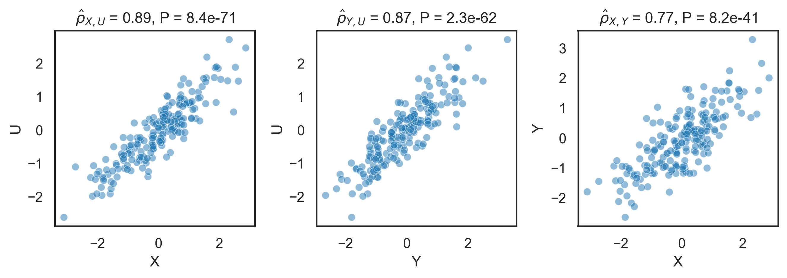
We want to discover this structure from observational data. Since both \(X\) and \(Y\) are caused by \(U\), a correlation is not very enlightening and will just return the fully connected graph:

A sensible way of going about it is to study the correlation between each pair of variables after adjusting for the remaining variable. If we assume all relationships are linear, these are called partial correlations. Partial correlations are designed to reveal direct relationships by removing the influence of confounding variables. Here is a naive implementation:

def pcorr_residuals(X: np.ndarray) -> np.ndarray:
    """
    Compute the matrix of partial correlations from the residuals of linear regression models.

    Parameters
    ----------
    X : np.ndarray
        The input data matrix.

    Returns
    -------
    np.ndarray
        The matrix of partial correlations.
    """

    n, p = X.shape

    residuals = np.empty((p, p), dtype=object)

    for i in range(p):
        for j in range(i + 1, p):
            covariates_indices = [k for k in range(p) if k != i and k != j]
            X_covars = X[:, covariates_indices]

            for target, excluded in [(i, j), (j, i)]:

                y = X[:, target]

                # fit a linear model
                beta, *_ = np.linalg.lstsq(X_covars, y, rcond=None)
                y_pred = X_covars @ beta

                # compute and center the residuals
                r = y - y_pred
                residuals[(target, excluded)] = r - r.mean()

    pcorr = np.eye(p)

    for i in range(p):
        for j in range(i + 1, p):

            res_1 = residuals[(i, j)]
            res_2 = residuals[(j, i)]
            corr = np.dot(res_1, res_2) / (np.linalg.norm(res_1) * np.linalg.norm(res_2))

            pcorr[i, j] = pcorr[j, i] = corr

    return pcorr

Partial correlations correctly identify that \(U\) is correlated with both \(X\) and \(Y\), and in turn that those are not correlated once we account for the effect of \(U\):

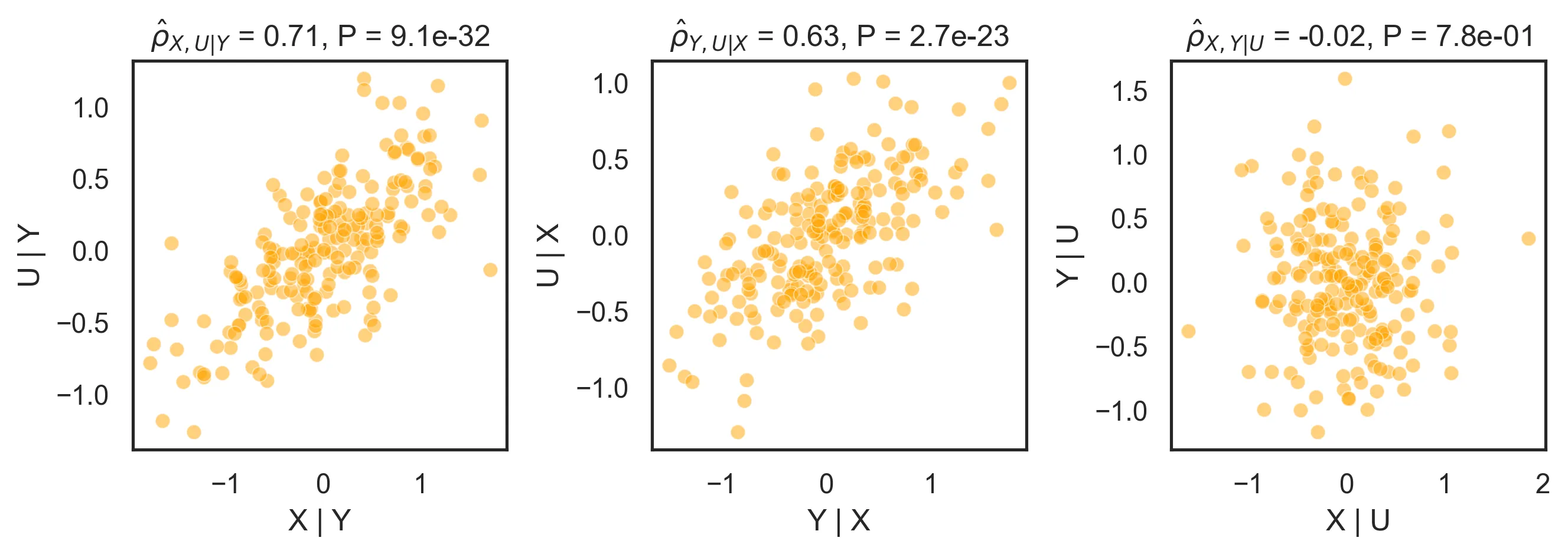
Note that while \(\hat{\rho}_{X, U} \approx \rho_{X, U} = 0.8944\), \(\hat{\rho}_{X, U \mid Y} \neq \rho_{X, U}\). This is because \(Y\) contains an additional noise term that makes the adjustment imperfect. Also note that we have identified the structure of the data (\(X - U - Y\)), but not its causal structure (\(X \rightarrow U \rightarrow Y\), \(X \leftarrow U \leftarrow Y\) or \(X \rightarrow U \rightarrow Y\)).

A downside of this approach is its computational complexity. For an \(n \times p\) input matrix:

• Memory complexity: \(\mathcal{O}(np^2)\), dominated by storing \({p \choose 2} = \mathcal{O}(p^2)\) residuals, each of length \(n\).
• Time complexity: \(\mathcal{O}(np^4)\), dominated by computing \({p \choose 2} = \mathcal{O}(p^2)\) least squares problems, each of complexity \(\mathcal{O}(np^2)\).

This is quite computational intensive, which will become a problem in real-world problems. Can we do better? Enter the precision matrix, a nice mathematical object to do this at scale.

The precision matrix

The covariance matrix of a set of random variables ties the variance and the covariance together. If \(\mathbf{X}\) is a column vector such that

then its associated covariance matrix \(\mathbf{\Sigma}\) is

Since always \(\text{Cov}(X_i, X_j) = \text{Cov}(X_j, X_i)\), \(\mathbf{\Sigma}\) is symmetric. It is, in fact, positive semi-definite (proof).

By normalizing the covariance matrix by dividing each item \(\mathbf{\Sigma}_{ij}\) by \(\sigma_{X_i} \sigma_{X_j}\), we obtain the correlation matrix:

Finally, the precision matrix \(\mathbf{\Sigma}^{-1}\) is the inverse of the covariance matrix, i.e., \(\mathbf{\Sigma} \mathbf{\Sigma}^{-1} = \mathbf{I}\). \(\mathbf{\Sigma}\) is not guaranteed to be invertible, and hence \(\mathbf{\Sigma}^{-1}\) may not exist. Let’s ignore this case for now, and jump to where things start getting interesting. \(\mathbf{\Sigma}^{-1}\) can be decomposed as follows:

where \(D\) is a normalization matrix:

The entries \(\rho_{X_., X_. \mid \dots}\) in the middle matrix are our precious partial correlations.

Estimating the precision matrix

Let’s revisit our motivating example equipped with our newfound knowledge: instead of fitting \(\mathcal{O}(p^2)\) linear models, let’s reach the same result using linear algebra. First, we will estimate the covariance matrix using the maximum likelihood approach. Then, we will invert it to obtain the precision matrix.

def pcorr_linalg(X: np.ndarray) -> np.ndarray: # (n, p) -> (p, p)
    """
    Compute the matrix of partial correlations from the covariance matrix.

    Parameters
    ----------
    X : np.ndarray
        The input data matrix.

    Returns
    -------
    np.ndarray
        The matrix of partial correlations.
    """

    n, p = X.shape

    # showing how the sausage is made
    # but could be replaced by covariance = np.cov(X, rowvar=False)
    centered_X = X - X.mean(axis=0)
    covariance = np.dot(centered_X.T, centered_X) / (n - 1)

    precision = np.linalg.inv(covariance)

    normalization_factors = np.sqrt(np.outer(np.diag(precision), np.diag(precision)))
    partial_correlations = - precision / normalization_factors

    return partial_correlations

This implementation is not only more compact, but has a more favorable computational complexity:

• Memory complexity: \(\mathcal{O}(p^2)\), dominated by the intermediate matrices.
• Time complexity: \(\mathcal{O}(np^2 + p^3)\), dominated by the computation of the covariance matrix and by the matrix inversion.

Furthermore, this implementation is vectorized which further boosts performance. As a quick benchmark, on a random \(1000 \times 100\) matrix, the original pcorr_residuals took 40.85 seconds; the updated pcorr_linalg took only 0.0007 seconds.

As with many elegant results in linear algebra, things start breaking down when our covariance matrix is ill-conditioned or outright non-invertible. In high-dimensional problems, \(\Sigma\) is non-invertible (and hard to estimate in the first place). In such cases, we could use the pseudoinverse matrix instead of the inverse. But that’s just a patch: we will get results, but we are outside of the theory and interpreting the results is not as straightforward. However, when the matrix is ill-conditioned, there is a potential path to salvation: regularization.

Regularized estimation

Adding a regularization step to the covariance matrix estimation will result in a better conditioned matrix. A common approach is shrinking our empirical covariance towards another matrix, the target:

where \(\alpha \in [0, 1]\) is a parameter and \(T\) is the target matrix, a highly structured matrix that encodes our assumption about what a true covariance matrix should look like. A possible and aggressive target matrix is a diagonal matrix, which encodes the assumption of zero covariance between variables. By upweighting the diagonal elements and downweighting the off-diagonal elements, this matrix will have a better condition than \(\Sigma_\text{MLE}\).

The problem becomes then tuning \(\alpha\). A common way to compute the \(\alpha\) is the Ledoit-Wolf shrinkage method, which finds the \(\alpha\) that minimizes the mean squared error between the real and the estimated matrix. Its scikit-learn implementation assumes that the target matrix is \(T = \mu I\), where \(\mu\) is the average variance.

Alternatively, we can use graphical lasso to estimate a sparse precision matrix. Conceptually, this is a bit easier to swallow: in many situations, most variables being conditionally uncorrelated is a valid assumption. The graphical lasso does just that; it is a penalized estimator of the precision matrix.

The \(- \lambda \|\mathbf{\Sigma}^{-1}\|_1\) term will favor sparse matrices, with a strength proportional to the magnitude of \(\lambda\). While tuning \(\lambda\) is in itself a challenge, a common approach is using cross-validation.

Let’s bring this point home by looking at a high-dimensional example (20 samples, 20 features).

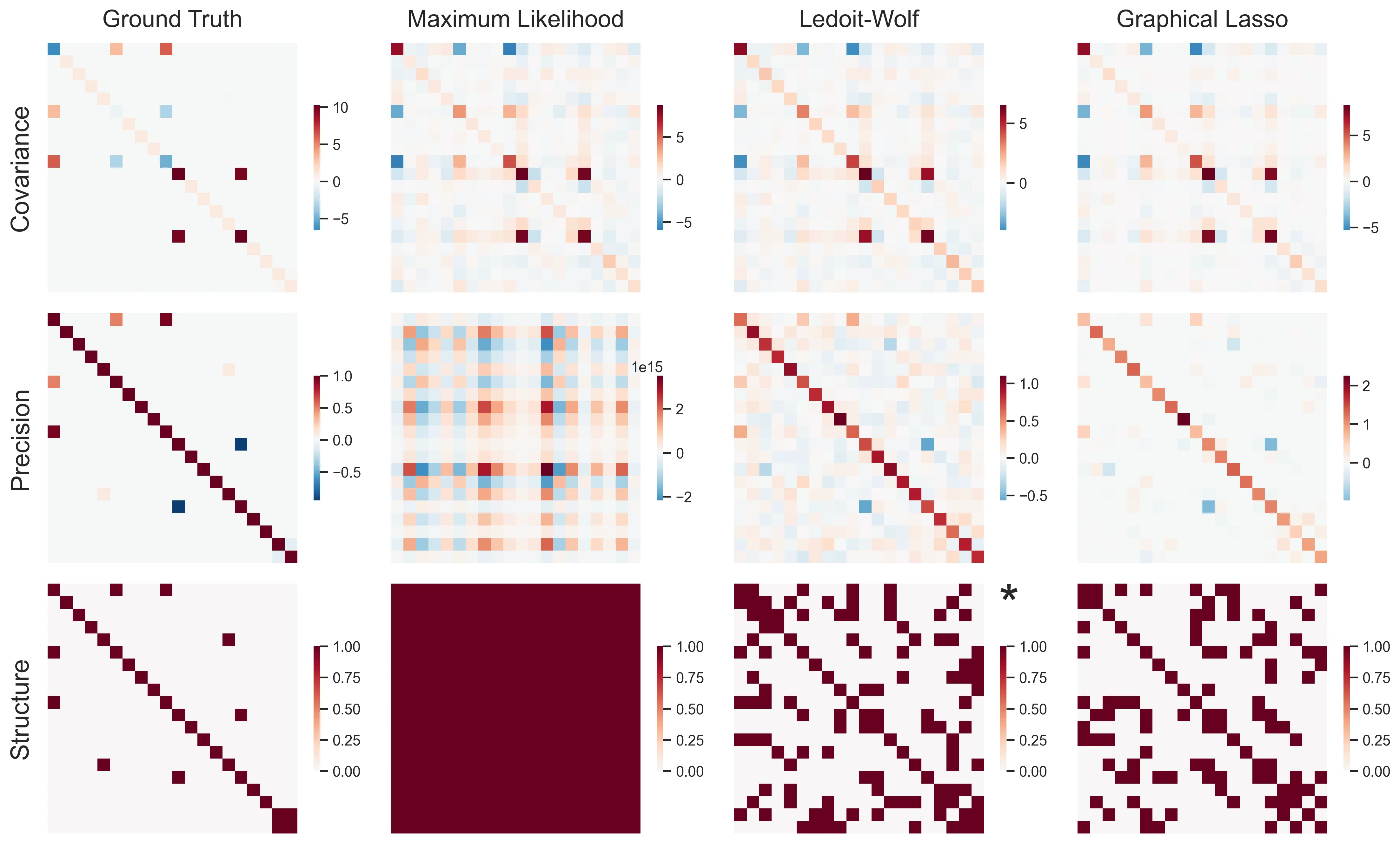
As we can see, maximum likelihood estimation absolutely fails. Due to the extremely ill-conditioned covariance matrix, the precision matrix is completely off scale, with values ranging from -1.8e+15 to 1.0e+15. Ledoit-Wolf succeeds at computing a sensible-looking precision matrix. But recovering a structure, e.g., by thresholding it, is quite a hard task. Last, graphical lasso is able to find a relatively sparse structure. While it is still far from the ground truth, it prunes away most of the spurious correlations and keeps most of the true links. As expected, most of the true links are larger in absolute value, and further pruning it would return something close to the true structure.

More than anything, this little exercise shows how hard this endeavour is, and serves as a good caution to high-dimensional statistics. Beware!

Conclusions

Under certain assumptions, the precision matrix helps us discover the internal structure of the data. When should we use what to estimate it?

1. Empirical inverse (MLE): fast and exact, but blows up if \(p\) approaches \(n\) or \(\hat Σ\) is singular. Use it when \(n \gg p\) and \(\hat Σ\) is well‑conditioned.
2. Shrinkage (Ledoit-Wolf): automatically picks \(\alpha\) to stabilize \(\hat Σ\), yielding a dense but well‑behaved precision. Use it when \(\frac p n\) is moderate.
3. Graphical Lasso (cross‑validated \(\lambda\)): trades off likelihood vs. sparsity to prune weak edges and reveal a parsimonious conditional‑independence network. Use it in high‑dimensional settings.