Independent Component Analysis
Cocktail parties make me anxious
Among spies, hackers and tabloids, independent component analysis (ICA) immediately brings to mind the cocktail party problem, the notorious signal processing problem it solves.
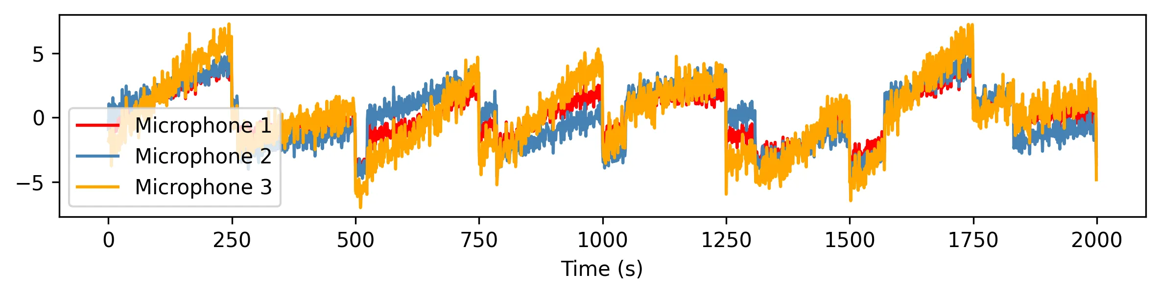
The problem reads as follows. A spy wants to snoop on all the conversations happening in a cocktail party. To that end, they strategically place multiple microphones across the room.
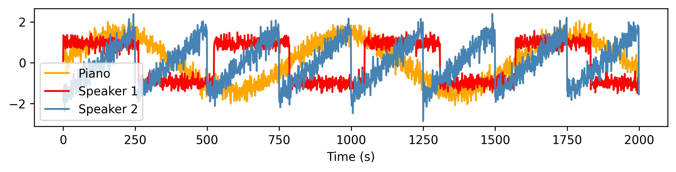
However, the party is quite busy: many conversations are ongoing, a piano plays in the background, guests gulp, waiters trot, glasses clink. Each microphone only captures a mixture of all these signals, which results in mostly incomprehensible gibberish.
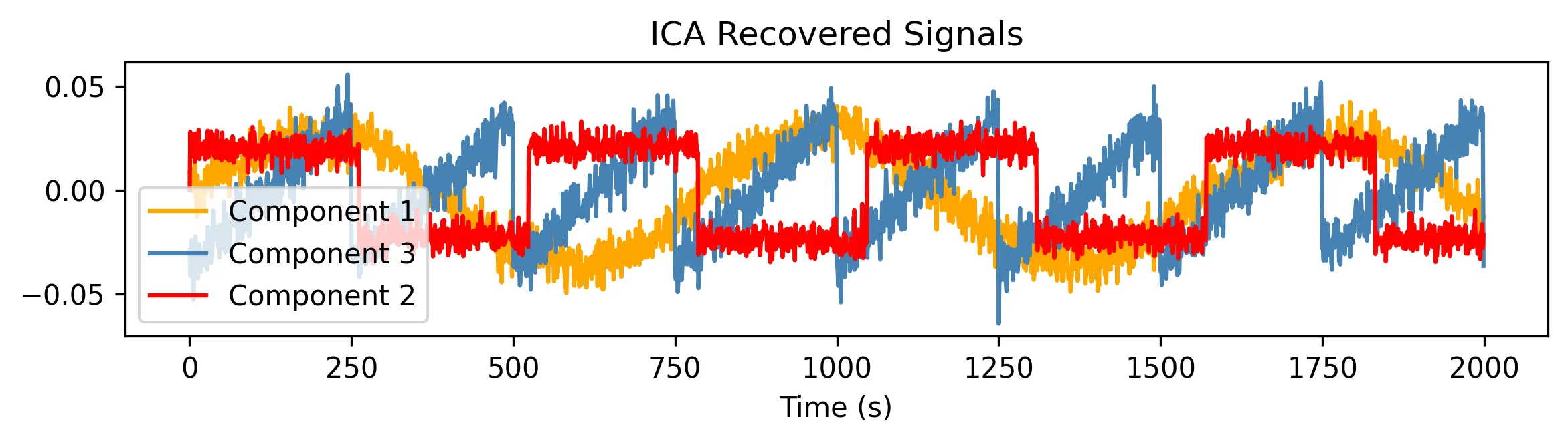
Other spies would get deterred, and move on to more persuasive ways of getting the information. But this is no ordinary spy. Armed with a secret weapon, ICA, they surgically extract the original conversations and save the world:
The geometry of ICA
The cocktail party problem is a good analogy for a common challenge in data science: untangling complex signals. Multidimensional datasets are somewhat redundant, consisting of complex mixtures of a relatively small number of latent factors. Distilling our dataset into that reduced number of dimensions can really help understand it better.
One way to go about it is matrix factorization, which decomposes our original matrix \(X\) into a product of matrices. Often the matrix is decomposed into two matrices: \(X = A S\). \(A\), the mixing matrix, represents a new vector basis. Since it’s a good descriptor of the geometry of the data, studying \(A\) can teach us something about it. \(S\), the score matrix, represents the coordinates of each datapoint in that new basis.
As you would have guessed, what “a good descriptor of the geometry of the data” is, exactly, is up for debate. But, in general, it should help with interpretability, data compression, or parsimony.
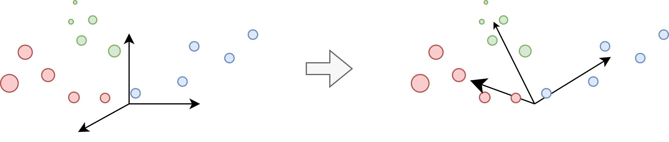
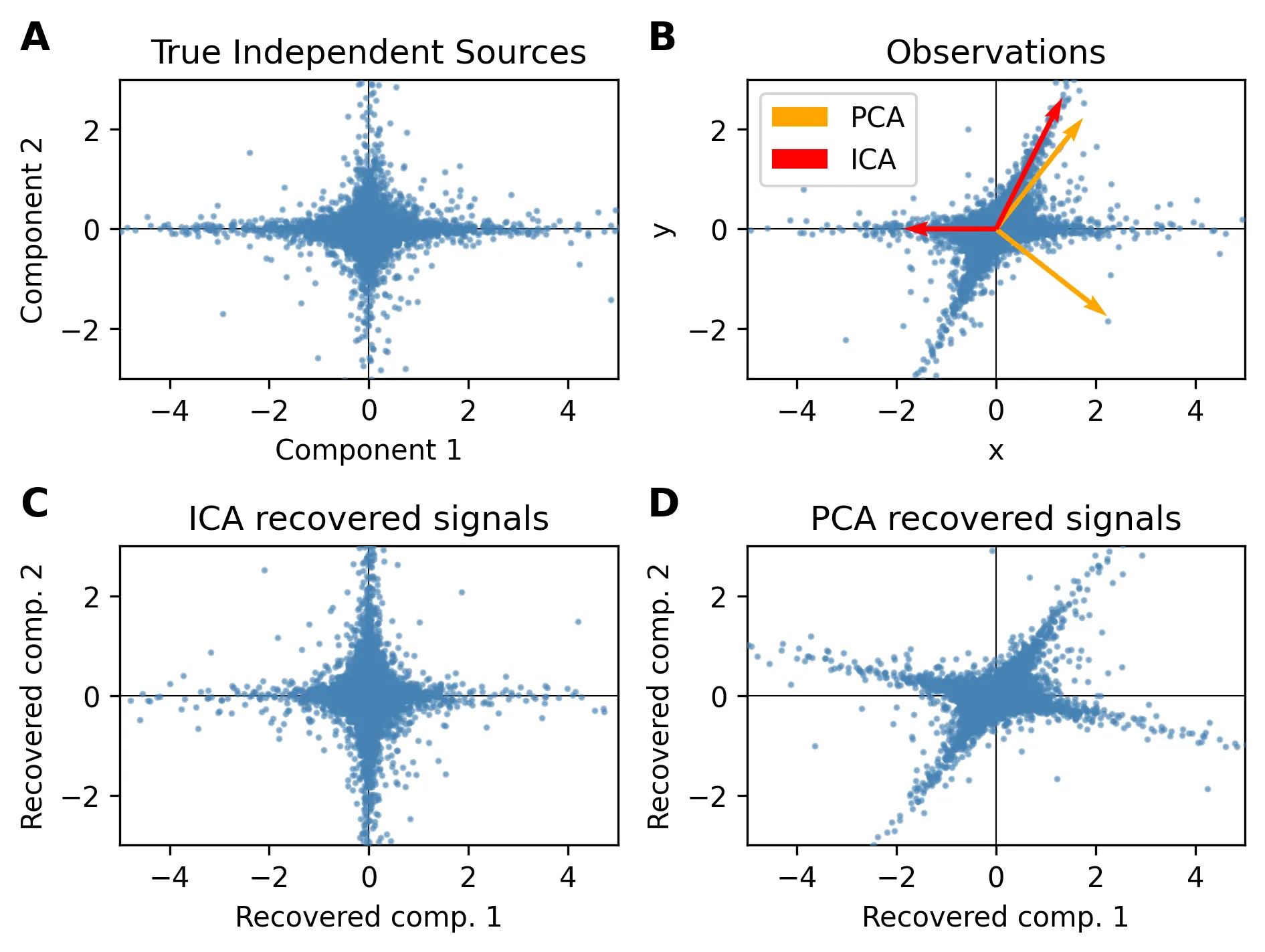
Unsurprisingly, many matrix factorizations have been proposed. A well-known one is the principal component analysis, or PCA. Geometrically speaking, PCA fits an ellipsoid to the data, and uses the axes of this ellipsoid as the basis for the new space. This is equivalent to PCA’s well-known interpretation: capturing the main axes of variation in the data. However, when our data has substructures that are not captured by the variance, PCA performs pretty poorly.

And this is where ICA shines:
How does ICA work?
PCA seeks a basis of uncorrelated components, since the axes of the ellipsoid need to be orthogonal. ICA goes one step further: it seeks a statistically independent basis.
More formally, ICA assumes the observed data is a mixture of the individual components. For instance, in the cocktail party, each component (e.g., the piano playing) is a vector indexed by time (\(s_j(t)\)). The components must meet two assumptions: non-Gaussianity and statistical independence. There is also an assumption that they are combined linearly to generate the observed data:
\[x_i = \sum_j a_{ij} s_j\]where \(a_{ij}\) is a constant, representing the relative contribution of each component.
We can arrange the observation vectors into a matrix, and think of it as a matrix factorization problem:
\[X = AS\]where \(A\) is called the mixing matrix and \(S\) the independent component matrix. The goal is to estimate both \(A\) and \(S\) from \(X\). To that end, ICA seeks a de-mixing matrix \(W\) such that:
\[S = W X\]The linearity assumption is key, since the central limit theorem tells us that the sum of independent random variables converges in distribution to a Gaussian. The magic lies here: our data needs to be more Gaussian than any of the individual components, and we will unmix them by seeking highly non-Gaussian components.
Specifically, we want \(W\) to maximize the non-Gaussianity of the recovered signals in \(S\). Once we have \(W\), computing \(A\) is straightforward, since \(W = A^{-1}\).
Quantifying non-Gaussianity
There are two popular ways of quantifying the non-Gaussianity of a distribution.
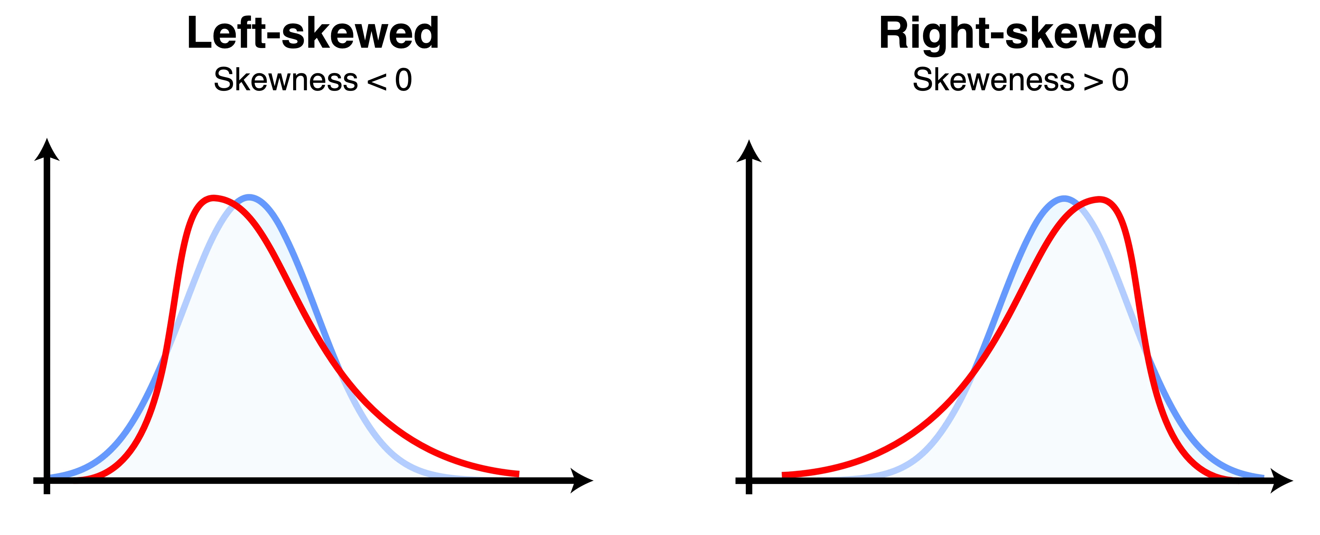
The first way consists in comparing the properties of the distribution called the moments. The first two moments, the mean and the variance, are not useful, since the data is usually standardized to have 0 mean and 1 variance. But the third and fourth moments (skewness and kurtosis, respectively) are frequently used:
- The skewness measures the asymmetry of the distribution. Gaussian distributions are famously symmetrical, and have a skewness of 0.
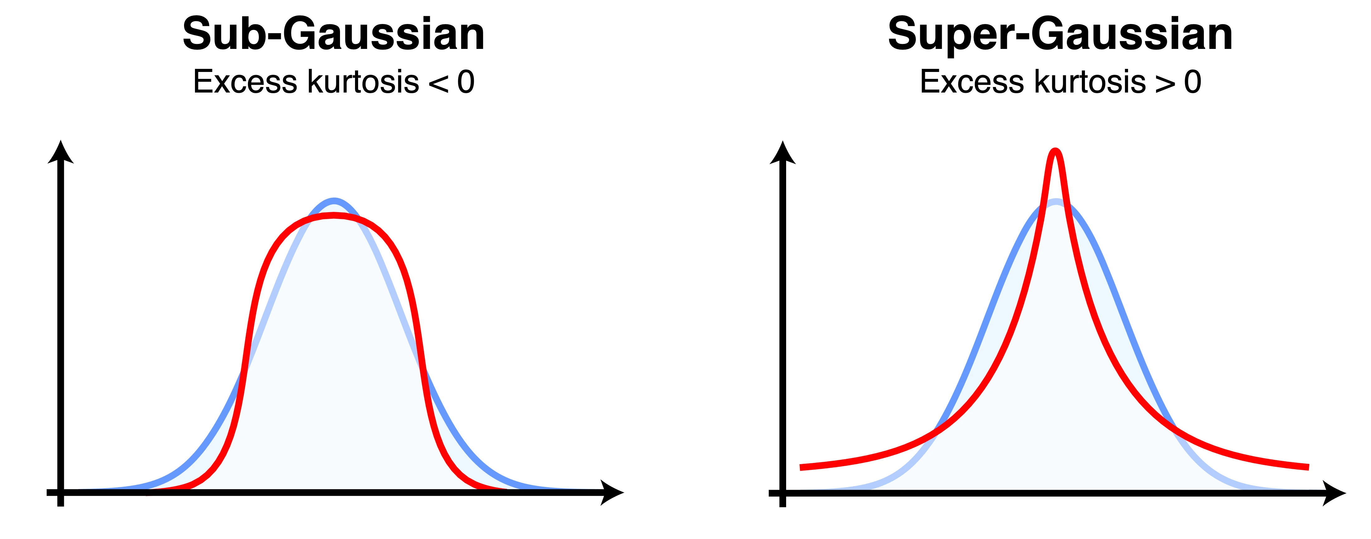
- The kurtosis measures the tailedness of the distribution. By comparing the kurtosis of our distribution relative to that of a normal distribution (excess kurtosis), we can estimate how non-Gaussian it is. The kurtosis is popular because it can be easily estimated from the data.
The second family involves using the entropy of the distribution. A fundamental theorem in information theory states that a Gaussian variable has the largest entropy among all random variables of equal variance. By computing the difference between the entropy of our distribution and that of a gaussian distribution of equal variance, we can estimate how non-Gaussian it is. This difference is called the negentropy.
Limitations
Before we continue, it’s important to acknowledge that ICA has some limitations.
First, it makes some strong assumptions about the data (linear mixing, non-Gaussianity, statistical independence) that may not hold in practice. If these assumptions are violated, the results of ICA may be misleading. For instance, if two or more components are Gaussian, ICA won’t be able to separate them.
Second, the solution matrices, \(A\) and \(S\) are not unique. Both the scale and the order of the components are arbitrary. In other words, scaling \(A\) by a constant and scaling \(S\) by the inverse of that constant yields the same product. Similarly, permuting the rows of \(A\) and the columns of \(S\) also yields the same product. Hence, two runs of ICA on the same data may yield different results, albeit they should be equivalent up to permutation and scaling.
Implementation
Let’s put the above into practice by aiming for the simplest, possibly most inefficient, implementation of ICA. We will work on an \(m \times n\) matrix \(X\), where \(m\) is the number of features and \(n\) the number of samples. Before we can apply ICA, we need to apply two preprocessing steps to \(X\):
- Centering, ensuring that each feature has a zero mean
- Whitening, ensuring that the features are uncorrelated and have unit variance. This vastly simplifies the ICA problem since it restricts the space of possible de-mixing matrices \(W\) to only orthogonal ones.
X_centered = X - np.mean(X, axis=0)
pca = PCA(whiten=True)
X_whitened = pca.fit_transform(X_centered)
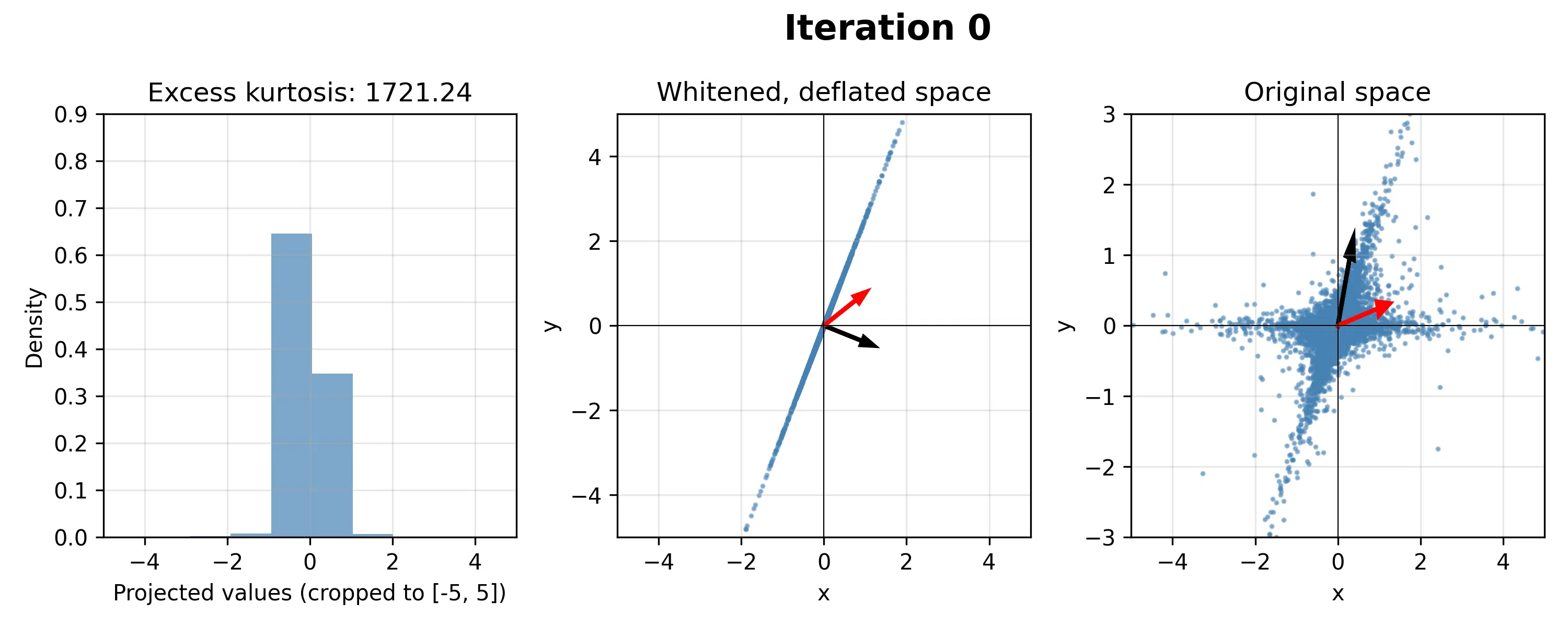
Now we will seek an \(m\)-dimensional vector \(\mathbf{w}_1\) that maximizes the non-Gaussianity of the independent component \(\mathbf{s}_{(1)} = X_{whitened} \mathbf{w}_1\). We will quantify non-Gaussianity using the excess kurtosis:
\[\operatorname{Kurtosis}(Y) = E\left[\left(\frac{Y - \mu}{\sigma}\right)^4\right] - 3.\]Since our data is centered and whitened, this simplifies to \(\operatorname{Kurtosis}(Y) = E\left[\left(Y\right)^4\right] - 3\).
We will use a biased sample estimator of the excess kurtosis:
\[\hat{K}(\mathbf{s}_{(1)}) = \frac 1 n \sum_{i=1}^n s_{(1)i}^4 - 3 = \frac 1 n \sum_{i=1}^n (\mathbf{x_{i*}}^\intercal \mathbf{w})^4 - 3.\]We will seek the \(\mathbf{w}_1\) that maximizes the kurtosis by gradient ascent. Hence, we need the first partial derivative of the kurtosis:
\[\frac { d \hat{K}(\mathbf{s}_{(1)}) } { d \mathbf{w}_1 } = \frac 1 n \sum_{i=1}^n 4 (\mathbf{x_{i*}}^\intercal \mathbf{w})^3 \mathbf{x_{i*}} = \frac 4 n \sum_{i=1}^n s_{(1)i}^3 \mathbf{x_{i*}}.\]Let’s implement this in Python:
STEP_SIZE = 1e-3
N_ITERATIONS = 50

# n = number of samples, m = number of features
n, m = X_whitened.shape

# Random initial weight vector
w1 = rng.rand(m)
w1 /= np.linalg.norm(w1) + 1e-10

for i in range(N_ITERATIONS):
    # Project data onto weight vector
    s = np.dot(X_whitened, w1)

    # Compute the gradient
    gradient = 4 / n * np.dot(np.pow(s, 3), X_whitened)

    # Update the weight vector
    w1 += STEP_SIZE * gradient

    # Normalize the weight vector
    w1 /= np.linalg.norm(w1) + 1e-10
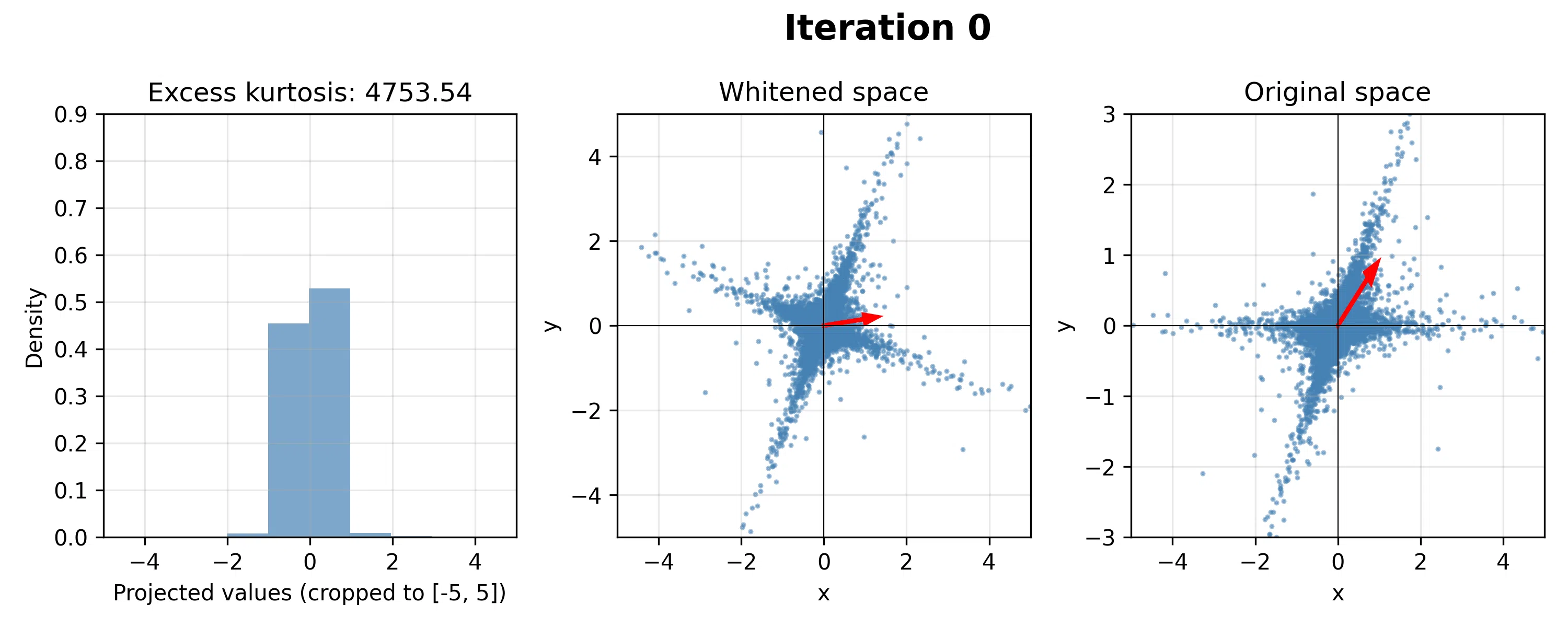
The algorithm converges pretty quickly:
Before repeating the process to find the second component, we need to ensure that it is statistically independent from the first component. We can achieve this through a deflation step, which removes the influence of already-found components from the data before searching for the next component. This process is conceptually similar to the Gram-Schmidt algorithm for creating orthogonal vectors.
X_deflated = X_whitened - np.outer(np.dot(X_whitened, w1), w1)
Deflation is good for illustration purposes, but too numerically unstable for practical use. A more robust approach is to use the symmetric decorrelation method, which ensures that keeps the data unchanged, and optimizes all components at once while keeping them orthogonal.
Then, we repeat:
# Random initial weight vector
w2 = rng.rand(m)
w2 /= np.linalg.norm(w2) + 1e-10

# Repeat gradient ascent to find second component
for i in range(N_ITERATIONS):
    s = np.dot(X_deflated, w2)
    gradient = 4 / n * np.dot(np.pow(s, 3), X_deflated)
    w2 += STEP_SIZE * gradient
    w2 /= np.linalg.norm(w2) + 1e-10
We could keep going by removing the influence of both the first and second components using the deflation steps, and running gradient ascent again to find the third component.
Our simple ICA gets the job done, but it is unstable and the results are not optimal, as we can see by comparing them with the results obtained in the ICA vs PCA comparison. If you want to play with ICA, FastICA is the way to go. It offers multiple improvements over my toy implementation, including a fast optimization process (fixed-point algorithm), solves all the components at once, and will even whiten the data for you.
Application: gene expression analysis
Ultimately, the reason I went down the ICA rabbit hole was not to eavesdrop in parties, but because of its applications in computational biology. Specifically, ICA is used to factorize gene expression matrices into a matrix containing groups of genes that work together (\(A\), the metagenes) and a matrix containing groups of similar samples (\(S\), the metasamples). Both can provide insights into the underlying biology:
- The metagenes are particularly useful when we can annotate them with the biological process they capture. We can do that by studying their overlap with known signatures or pathways, or finding commonalities among the genes’ properties.
- The metasamples can be helpful if we have other information about the samples (e.g., clinical records) that help us understand what each set of samples have in common.
Teschendorf et al. (2007) provides an example for both. While other matrix factorization algorithms are common, ICA is one of the best, making it an essential tool in the computational biologist’s toolbox.