Cross-entropy. Intuition and applications.
The secret sauce of machine learning
In pop science, entropy is considered a measure of disorder: a system has high entropy when it is disordered (e.g., my college bedroom), and low entropy when it is ordered (e.g., a chocolate box). This meaning probably has its roots in thermodynamics, where my college bedroom was evidence of the universe getting ever closer to its heat death.
But for us, entropy is not (only) about messy bedrooms, but about messy data. That’s why I will focus on Shannon’s entropy \(H(P)\), which is a property of a probability distribution \(P\). For a discrete random variable:
\[H(P) = \sum_x P(x) \log_2 \frac{1}{P(x)}.\]As stated, using the binary logarithm, entropy is measured in bits; when using the natural logarithm instead, the unit of measure is nats. From here on, \(\log\) means \(\log_2\).
What does entropy really mean?
In a nutshell, entropy is the average surprise we’ll experience when observing a realization of \(P\): if an outcome is rare (\(P(x)\) is small), observing it should be quite surprising (\(\log \frac{1}{P(x)}\) is large); if it is very common, the surprise should be low.
A more tangible interpretation of entropy links it to the encoding of a message. Imagine we want to encode the outcome of a probability distribution. We observe an outcome and want to unambiguously communicate it to a friend. For instance, let’s say the weather in my city follows the following probability distribution:
| Weather | Probability |
|---|---|
| Cloudy | 0.5 |
| Rainy | 0.4 |
| Sunny | 0.1 |
(Yes, I live in London.)
For easier computations, let’s assume that probabilities remain independent and constant over time. Which, again, isn’t too far from my reality. More formally, the outcomes are independent and identically distributed.
Every morning, I look out the window exactly at 9am, and send my friend the weather report. Our first instinct is probably to just text them “cloudy”, “rainy” or “sunny” as appropriate. If we encode these strings in ASCII:
| Weather | Probability | Codeword | Codeword length |
|---|---|---|---|
| Cloudy | 0.5 | 011000110110110001101111011101010110010001111001 | 48 |
| Rainy | 0.4 | 0111001001100001011010010110111001111001 | 40 |
| Sunny | 0.1 | 0111001101110101011011100110111001111001 | 40 |
In the long term, the average message will take \(0.5 \times 48 + 0.4 \times 40 + 0.1 \times 40 = 44\) bits. Not a big deal I guess… But we can do much better! Why waste time say lot word when few word do trick? For instance, we could associate each string to an integer or an emoji (8 bits). But we can do even better than that, we can generate our own codewords. To this end, we need to generate a prefix code, i.e., one in which no codeword can prefix another.
The Huffman coding is a common solution to this problem which significantly shortens our average message by leveraging our knowledge of \(P\):
| Weather | Probability | Codeword | Codeword length |
|---|---|---|---|
| Cloudy | 0.5 | 0 | 1 |
| Rainy | 0.4 | 10 | 2 |
| Sunny | 0.1 | 11 | 2 |
Huffman coding
Huffman coding builds an optimal prefix code for a known distribution. Here’s how it works for our weather example:
-
Start with probabilities:
Weather Probability Cloudy 0.5 Rainy 0.4 Sunny 0.1 -
Merge lowest pairs: Combine Sunny (0.1) and Rainy (0.4) → node with weight 0.5. Then combine with Cloudy (0.5) → final tree.
-
Assign bits: Traverse the tree, assigning 0/1 at each split.
Weather Codeword Cloudy 0 Rainy 10 Sunny 11
Huffman coding guarantees the shortest average length for any prefix code based on the true distribution.
This is much better: we have gone from 44 bits to \(0.5 \times 1 + 0.4 \times 2 + 0.1 \times 2 = 1.5\) bits on average. Of course, for this to be possible, we need to have access to the true weather distribution. Otherwise, our bit allocation won’t be optimal.
Are we satisfied yet? Not quite. Despite Huffman being optimal, our message length will be the same on rainy days and on sunny days. However, rainy days are 4 times more common! The core problem is that our messages have an integer length, and we would need fractional lengths to do better. But we can do better if we make some compromises. Imagine we only want to batch-send the weather report every 10 days. Then, there are \(3^{10}\) possible sequences of 10 days. The most likely one is a streak of ten cloudy days, which occurs with probability \(0.5^{10}\). Consequently, the Huffman coding assigns a much shorter codeword to this string than to the most unlikely string, a streak of ten sunny days:
| 10-day weather | Probability | Codeword | Codeword length |
|---|---|---|---|
| CCCCCCCCCC | 9.77e-04 | 0111001010 | 10 |
| CCCCCCCCCR | 7.81e-04 | 0000101101 | 10 |
| CCCCCCCCRC | 7.81e-04 | 0000101110 | 10 |
| … | … | … | … |
| SSSSSSSSSR | 4.00e-10 | 0111001001100000001100111110100 | 31 |
| RSSSSSSSSS | 4.00e-10 | 11000100010100011010000101101111 | 32 |
| SSSSSSSSSS | 1.00e-10 | 11000100010100011010000101101110 | 32 |
The average length of this code is 13.64 bits, or 1.364 bits per day. Batching outcomes together allows us to spend only fractions of a bit. And it’s easy to see how, if we kept batching more and more days together, each single day would require less and less bits.
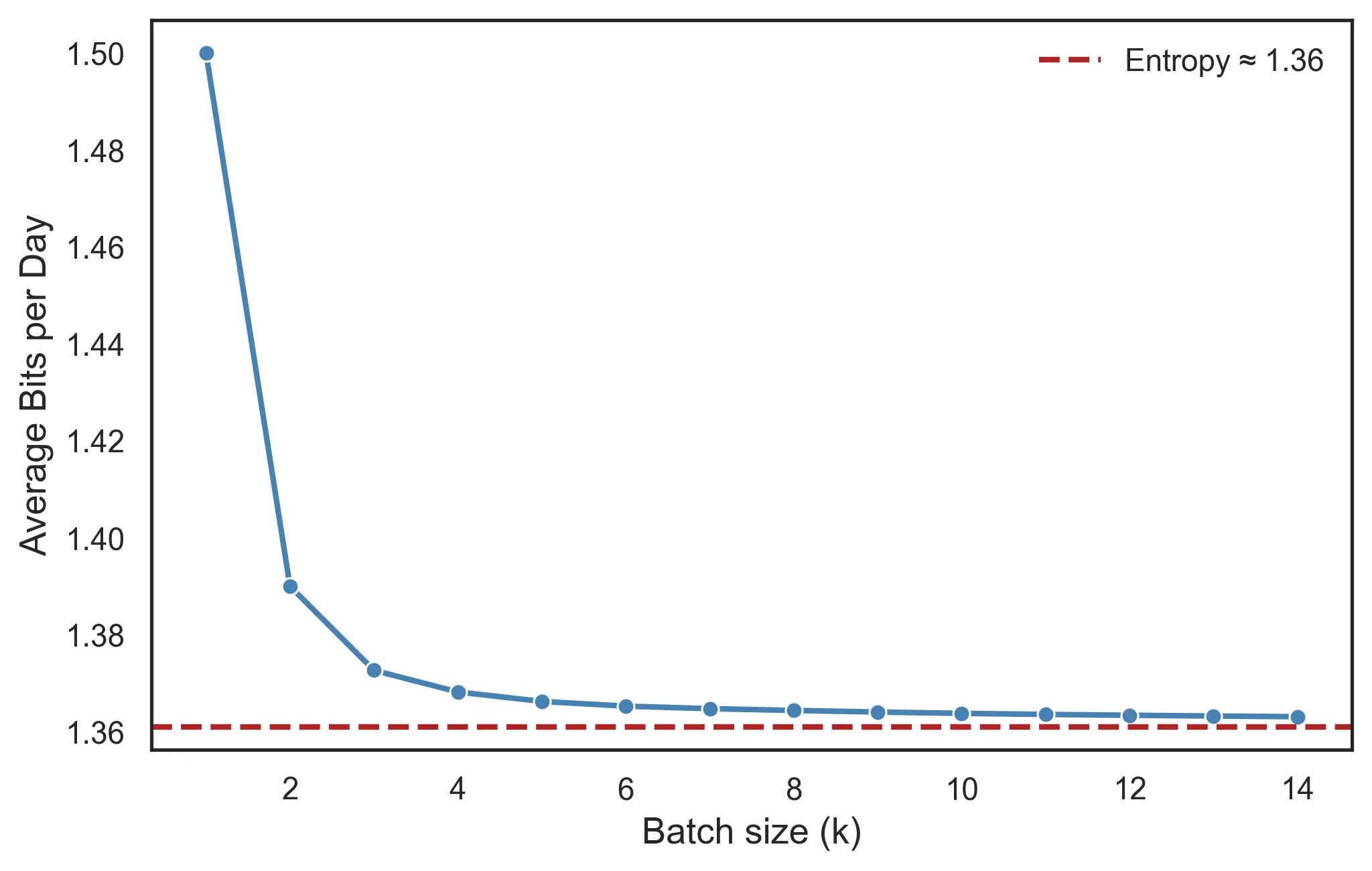
And this brings us to the key point: entropy represents the lower bound for the average message length required to optimally encode each outcome of a random process. Even with the best encoding we can come up with and incredibly large batches, we can’t compress the message below the entropy limit. In the case of our distribution:
\[H(P) = 0.5 \times \log \frac 1 {0.5} + 0.4 \times \log \frac 1 {0.4} + 0.1 \times \log \frac 1 {0.1} = 1.361 \text{ bits}\]The Huffman encoding was doing pretty well after all!
But why logarithms?
All this is fine, but a lingering question remains: what’s the logarithm of the probability doing there? Why aren’t we using any other transformation of the probability?
Imagine the space of all possible codewords of a prefix code. If we decide to use the codeword “0”, every other codeword needs to start by “1”; that choice cost us half of all possible codewords. Hence, if we are going to spend that precious codeword into one outcome, it better happen at least half the time. Note that \(- \log 0.5 = 1\). Similarly, a codeword like “00” still allows for words prefixed by “01”, “10” and “11”; it cost us only one fourth of the space. Note that \(- \log 0.25 = 2\).
\(- \log P(x)\) gives us the optimal length of an outcome’s codeword.
Cross-entropy
We just saw how knowing the underlying probability distribution gave us an edge in encoding the outcomes efficiently. However, here in the real world we rarely have access to true probability distributions, if such a thing even exists. At most, we have access to our best guess of what the true probability distribution is. And these guesses are rarely completely correct.
For instance, we rely on very complex models to accurately predict the weather. But let’s leave those aside, and use the simple model (\(Q_\text{Barcelona}\)) and associated Huffman code I developed for Barcelona’s weather:
| Weather | Probability | Codeword | Codeword length |
|---|---|---|---|
| Cloudy | 0.2 | 11 | 2 |
| Rainy | 0.1 | 10 | 2 |
| Sunny | 0.7 | 0 | 1 |
As you can imagine, after moving to London, my model of the weather was not that useful. In fact, I often experienced surprise, as outcomes that should be rare happened often. In consequence, when using this code in London, my average message took up 1.9 bits.
Entropy quantified our average surprise when observing a distribution’s outcomes while knowing the true distribution. Similarly, the cross-entropy measures our surprise when observing a distribution’s outcomes while only having a model of the true distribution. If \(P\) is the true distribution and \(Q\) is our model:
\[H(P, Q) = \sum_x P(x) \log \frac{1}{Q(x)}.\]Just like entropy, \(\log \frac{1}{Q(x)}\) measures the degree of surprise we expect as per our model, which is weighted by the actual frequency with which we observe the outcome. It is also measured in bits.
Note that order matters! \(H(P, Q) \neq H(Q, P)\).
Why theory and practice can differ
The cross-entropy of my model \(Q_\text{Barcelona}\) on the London weather is:
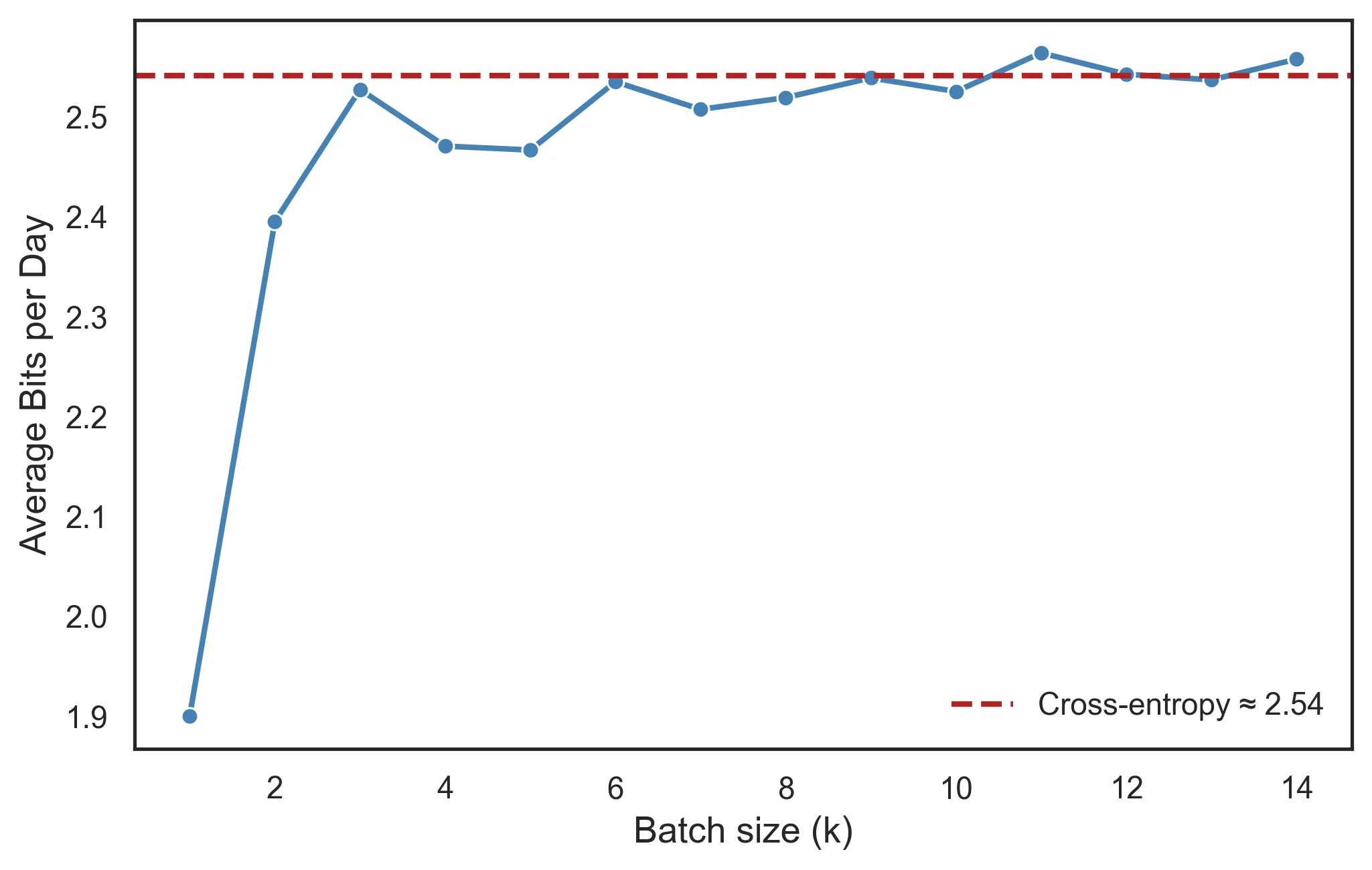
\[H(P_\text{London}, Q_\text{Barcelona}) = 0.5 \times \log \frac 1 {0.2} + 0.4 \times \log \frac 1 {0.1} + 0.1 \times \log \frac 1 {0.7} \approx 2.54 \text{ bits}.\]This is higher than the average message length of 1.9 bits. Contrary to entropy, which is a hard-limit, our model can do better than cross-entropy. This is because the cross-entropy leverages (optimal) fractional lengths, but our Huffman codes use non-fractional lengths, underestimating some outcomes and overestimating others:
| Weather | P | Codeword length | Q-optimal codeword length | Extra (\(+\))/Saved (\(-\)) bits |
|---|---|---|---|---|
| Cloudy | 0.5 | 2 | 2.32 | \(-0.32 \times 0.5 = -0.16\) |
| Rainy | 0.4 | 2 | 3.32 | \(-1.32 \times 0.4 = -0.53\) |
| Sunny | 0.1 | 1 | 0.51 | \(0.49 \times 0.1 = 0.05\) |
Notice how we’re saving a ton of bits on cloudy and rainy days; we got lucky. If we batch our weather reports, we get closer to encoding individual outcomes with fractional bits. Using the 10-day Barcelona code to report London weather, the average length of my message was \(2.53 \text{ bits}\), which is much closer to \(H(P, Q) \approx 2.54 \text{ bits}\). The cross-entropy is a lower bound if and only if we achieve the optimal coding for \(Q\).
Why does this all matter?
After a few years in London my model became quite accurate, to the extent that \(Q_\text{London} \approx P_\text{London}\):
\[H(P_\text{London}, Q_\text{London}) = 0.5 \times \log \frac 1 {0.5} + 0.4 \times \log \frac 1 {0.4} + 0.1 \times \log \frac 1 {0.1} \approx 1.36 \text{ bits}.\]This is an important result (the Gibbs’ inequality):
\[H(P, Q) \geq H(P, P) = H(P)\]Kullback-Leibler (KL) divergence
Since entropy is the lower bound for cross-entropy, the difference between both informs us about how well our model reflects the true distribution. This difference is also so important that it has its own name: Kullback-Leibler (KL) divergence.
\[D_{KL}(P || Q) = H(P, Q) - H(P)\]It can be interpreted as the cost of being wrong: how many extra bits we need to spend because our model departs from the true distribution.
Ultimately, this is why I went down this rabbit hole. We’ve covered distributions, processes, and encoding. But machine learning is one of the most important applications of cross-entropy via the cross-entropy loss. During model training, many machine learning algorithms minimize the cross-entropy between the learned probability distribution (like \(P(Y \mid X)\) or \(P(X, Y)\)) and the one observed in the data.
Let’s bring this point home by revisiting our weather model one last time. In this case, we want a model to predict tomorrow’s weather using some sensible variables (like today’s weather, temperature, humidity and wind), encapsulated into a vector \(x\). After some complex calculations it emits a probability vector \(q(x) = [q_C, q_R, q_S]\). Say, for a given day, it predicts \(q(x) = [0.35, 0.6, 0.05]\). Then, the day arrives, and we observe the true outcome: \(p = [1, 0, 0]\). Turns out our model was quite wrong!
Note that \(p\) is the one-hot (empirical) distribution on the observed class, not the true generative \(P\), and \(q\) is just the model’s prediction for this example, not the overall distribution \(Q\)!
The cross-entropy loss has a familiar form:
\[\mathcal{L}(p,q(x)) = 1 \times \log\frac{1}{q_C} + 0 \times \log\frac{1}{q_R} + 0 \times \log\frac{1}{q_S} = \log\frac{1}{q_C} = - \log q_C.\]Or, more generally:
\[\mathcal{L}(p, q(x)) = -\sum_{i=1}^K p_i \log q(x)_i = -\log q(x)_y.\]where \(K\) is the number of classes, and \(y\) is the index of the true class (\(1\) in our example, corresponding to class \(C\)).
The model will consequently update its parameters to minimize this loss, also known as log-loss. Minimizing it is equivalent to maximizing the probability of the data. During training we minimize the average of this loss over the whole training dataset \(\mathcal{D}\):
\[\mathcal{L} = \mathbb{E}_{(x,y) \sim \mathcal{D}} \bigl[-\log q(x)_y \bigr] = -\frac{1}{N}\sum_{i=1}^N \log q(x^{(i)})_{y^{(i)}}.\]And that’s the objective in its entirety: to adjust the model’s parameters until it is, on average, least surprised by the correct answer. At least until it sees the test set…